Maximum Principle Based Algorithms for Deep Learning
Qianxiao Li [email protected]
Institute of High Performance Computing Agency for Science, Technology and Research
1 Fusionopolis Way, Connexis North, Singapore 138632
Long Chen [email protected]
Peking University Beijing, China, 100080
Cheng Tai [email protected]
Beijing Institute of Big Data Research and Peking University
Beijing, China, 100080
Weinan E [email protected]
Princeton University Princeton, NJ 08544, USA,
Beijing Institute of Big Data Research and Peking University
Beijing, China, 100080
Editor:Yoshua Bengio
Abstract
The continuous dynamical system approach to deep learning is explored in order to devise alternative frameworks for training algorithms. Training is recast as a control problem and this allows us to formulate necessary optimality conditions in continuous time using the Pontryagin’s maximum principle (PMP). A modification of the method of successive approximations is then used to solve the PMP, giving rise to an alternative training algo-rithm for deep learning. This approach has the advantage that rigorous error estimates and convergence results can be established. We also show that it may avoid some pit-falls of gradient-based methods, such as slow convergence on flat landscapes near saddle points. Furthermore, we demonstrate that it obtains favorable initial convergence rate per-iteration, provided Hamiltonian maximization can be efficiently carried out - a step which is still in need of improvement. Overall, the approach opens up new avenues to attack prob-lems associated with deep learning, such as trapping in slow manifolds and inapplicability of gradient-based methods for discrete trainable variables.
Keywords: deep learning, optimal control, Pontryagin’s maximum principle, method of successive approximations
1. Introduction
Supervised learning using deep neural networks has become an increasingly successful tool in modern machine learning applications (Bengio, 2009; Schmidhuber, 2015; LeCun et al.,
c
2015; Goodfellow et al., 2016). Efficient training methods of very deep neural networks, however, remain an active area of research. The most commonly applied training method is stochastic gradient descent (Robbins and Monro, 1951; Bottou, 2010) and its variants (Duchi et al., 2011; Zeiler, 2012; Kingma and Ba, 2014; Johnson and Zhang, 2013), where incremen-tal updates to the trainable parameters are performed using gradient information computed via back-propagation (Kelley, 1960; Bryson, 1975). While efficient to implement, the in-cremental updates to the parameter tend to be slow, especially in the initial stages of the training. Moreover, other than the computation of gradients through back-propagation, the specific structure of deep neural networks is not exploited. These observations point to the question of whether there exists alternative training methods tailored to deep neural networks.
In a series of papers, we introduce an alternative approach by exploring the optimal con-trol viewpoint of deep learning (E, 2017). Our focus will be on ideas and algorithms derived from the powerful Pontryagin’s maximum principle (Boltyanskii et al., 1960; Pontryagin, 1987), which has two major components: the Hamiltonian dynamics and the condition that at each time the optimal parameters maximize the Hamiltonian. The second component suggests that optimization can be performed independently at different layers. One can also derive an explicit error control estimate based on the maximum principle (see Lemma 2 be-low).
In this first paper, we will consider the simplest context in which the deep neural net-works are replaced by continuous (or discretized) dynamical systems, and devise numerical algorithms that are based on the optimality conditions in the Pontryagin’s maximum prin-ciple. This leads to a new approach for training deep learning models that have certain advantages, such as fast initial descent and resilience to stalling in flat landscapes. An additional advantage is that one has a good control of the error through explicit estimates. The rest of the paper is organized as follows. In Section 2, we present a dynamical systems viewpoint of function approximation and deep learning. We then discuss the nec-essary optimality conditions, which is the well-known Pontryagin’s maximum principle. In Section 3 and 4, we discuss numerical methods to solve the necessary conditions and ob-tain error estimates and convergence guarantees. Using benchmarking examples, we then compare our method with traditional gradient-descent based methods for optimizing deep neural networks in Section 5. In Section 6, we discuss and compare our work with existing literature. Conclusion and outlook are given in Section 7.
2. Function Approximation by Dynamical Systems
We start with a description of the (continuous) dynamical systems approach to machine learning (see E 2017). The essential task of supervised learning is to approximate some function
F :X → Y
which maps inputs inX ⊂Rd(e.g. images, time-series) to labels inY (categories, numerical predictions). Given a collection of K sample input-label pairs {xi, yi = F(xi)}K
i=1, one
differential equations
˙
Xti =f(t, Xti, θt), X0i =xi, 0≤t≤T, (1) where θ : [0, T] → Θ ⊂ Rp, represents the control (training) parameters and X
t = (Xt1, . . . , XtK) ∈ Rd×K for all t ∈ [0, T]. The form of f is chosen as part of the machine learning model. For example, in deep learning, f is typically the composition (in either order) of a linear transformation and a component-wise nonlinear function (the activation function). For the solution to (1) to exist for any θ, we shall assume hereafter that f and ∇xf are continuous in t, x, θ. Note that weaker but more complicated conditions can be considered (Clarke, 2005). For the ith input sample, the prediction of the “network” is a deterministic transformation of the terminal state g(XTi) for some g : Rd → Y, which we can view collectively as a function of the initial state (input) xi and the control parameters (weights)θ. The dynamics (1) are decoupled across samples except for the dependence on the controlθ. We shall consider quite a general space of controls
U :={θ: [0, T]→Θ :θ is Lebesgue measurable}.
The aim is to selectθ fromU so thatg(Xi
T) most closely resemblesyi fori= 1, . . . , K. To this end, we define a loss function Φ :Y × Y →R which is minimized when its arguments are equal, and we consider minimizingP
iΦ(g(xiT), yi). Sinceg is fixed, we shall absorb it into the definition of the loss function by defining Φi(·) := Φ(·, yi). Then, the supervised learning problem in our framework is
min θ∈U
K
X
i=1
Φi(XTi) +
Z T
0
L(θt)dt,
˙
Xti =f(t, Xti, θt), X0i =xi, 0≤t≤T, i= 1, . . . , K, (2)
whereL: Θ→Ris a running cost, or the regularizer1. We note here that alternatively, we can formulate the supervised learning problem more generally in terms of optimal control in function spaces, see Appendix A.
Problem (2) is a special case of a class of general optimal control problem for ordinary differential equations (Bertsekas, 1995; Athans and Falb, 2013). The advantage of this formulation is that we can write down and study the optimality conditions of (2) entirely in continuous time and derive numerical algorithms that can subsequently be discretized. In other words, weoptimize, then discretize, as opposed to the traditional reverse approach in deep learning.
As was suggested in E (2017), deep residual networks (He et al., 2016) can be considered as the forward Euler discretization of the continuous approach described above. In this connection, the algorithms presented in this paper can also be formulated in the context of deep residual networks. For general deep neural networks, although one can also formulate similar algorithms, it is not clear at this moment that PMP holds and these algorithms are valid (e.g. converge to the right solution) in the general setting. This issue will be studied in future work.
1. We can also makeL depend onXt, but for simplicity of presentation and the fact that most current
The optimization problem (2) can be solved by first discretizing it into a discrete problem (a feed-forward neural network) and then applying back propagation and gradient descent approaches commonly used in deep learning. However, here we will present an alternative approach. Hereafter, for simplicity of notation we shall set K = 1 drop the scripts i on all functions, noting that analogous results can be obtained in the general case since the dynamics and loss functions are decoupled across samples. Equivalently, we can think of this as effectively concatenating allKsample inputs into a single input vector of dimension
d×K and redefine our dynamics accordingly. Hence, all results remain valid if we perform full-batch training. The case of mini-batch training is discussed in Section 4.3.
2.1 Pontryagin’s Maximum Principle
In this section, we introduce a set of necessary conditions for optimal solutions of (2), known as the Pontryagin’s Maximum Principle (PMP) (Boltyanskii et al., 1960; Pontryagin, 1987). This shall pave way for an alternative numerical algorithm to train (2) and its discrete-time counter-part.
To begin with, we define the HamiltonianH : [0, T]×Rd×
Rd×Θ→R given by
H(t, x, p, θ) :=p·f(t, x, θ)−L(θ).
Theorem 1 (Pontryagin’s Maximum Principle) Letθ∗ ∈ U be an essentially bounded optimal control, i.e. a solution to (2) with ess supt∈[0,T]kθt∗k∞ < ∞ (ess sup denotes the
essential supremum). Denote by X∗ the corresponding optimally controlled state process. Then, there exists an absolutely continuous co-state process P∗ : [0, T]→Rd such that the
Hamilton’s equations
˙
Xt∗ =∇pH(t, Xt∗, Pt∗, θt∗), X0∗ =x, (3) ˙
Pt∗ =−∇xH(t, Xt∗, Pt∗, θ∗t), PT∗ =−∇Φ(XT∗), (4)
are satisfied. Moreover, for eacht∈[0, T], we have the Hamiltonian maximization condition
H(t, Xt∗, Pt∗, θt∗)≥H(t, Xt∗, Pt∗, θ) for all θ∈Θ. (5)
The proof of the PMP and its variants can be found in any optimal control theory reference, e.g. Athans and Falb (2013); Bertsekas (1995); Liberzon (2012). Some gener-alizations can be found in Clarke (2005) and references therein. For example, the re-quirement of the continuity of f with respect to t can be replaced by a much weaker measurability requirement if one assumes more conditions on ∇xf. In the statement of Theorem 1, we omitted a technicality involving an abnormal multiplier: the terminal con-dition for P∗ should be PT∗ = −λ∇Φ(XT∗) and the Hamiltonian should be defined as
A few remarks are in order. First, Equation 3, 4 and 5 allow us to solve for the unknowns
X∗, P∗, θ∗ simultaneously as a function of t. In this sense, the resulting optimal control θ∗
is open-loop and is not in a feed-back form θt∗ =θ∗(Xt∗). The latter is of closed-loop type and are typically obtained from dynamic programming and the Hamilton-Jacobi-Bellman formalism (Bellman, 2013). In this sense, the PMP gives a weaker control. However, open-loop solutions are sufficient for neural network applications, where the trained weights and biases are fixed and only depend on the layer number and not the inputs.
PMP can be regarded as a (highly non-trivial) generalization of the calculus of variations to non-smooth settings (since we only assumeθ∗ to be measurable). Perhaps more familiar to the optimization community, the PMP is related to the Karush-Kuhn-Tucker (KKT) conditions for non-linear constrained optimization. Indeed, we can view (2) as a non-linear program over the function space U where the constraint is the ODE (1). In this sense, the co-state process P∗ plays the role of a continuous-time analogue of Lagrange multipliers. The key difference between the PMP and the KKT conditions (besides the lack of inequality constraints on the state) is the Hamiltonian maximization condition (5), which is stronger than a typical first-order condition that assumes smoothness with respect to θ
(e.g. ∇θH = 0). In particular, the PMP says that H is not only stationary, but globally maximized at an optimal control - which is a much stronger statement ifH is not concave. Moreover, the PMP makes minimal assumptions on the parameter space Θ; the PMP holds even whenf is non-smooth with respect to θ, or worse, when Θ is a discrete subset ofRp.
Last, we emphasize that the PMP is only a necessary condition, hence there can be cases where solutions to the PMP is not actually globally optimal for (2). Nevertheless, in practice the PMP is often strong enough to give good solution candidates, and when certain convexity assumptions are satisfied the PMP becomes sufficient (Bressan and Piccoli, 2007). In the next section, we will discuss numerical methods that can be used to solve the PMP.
3. Method of Successive Approximations
Now, our strategy is to devise numerical algorithms for training (2) via solving the PMP (Equation 3, 4 and 5). We derive and analyze algorithms entirely in continuous time, which allows us to characterize errors estimates and convergence in a more transparent fashion.
3.1 Basic MSA
Observe that (3) is simply the equation
˙
Xt∗=f(t, Xt∗, θ∗t),
and is independent of the co-stateP∗. Therefore, we may proceed in the following manner. First, we make an initial guess of the optimal control θ0 ∈ U. For each k= 0,1,2, . . ., we first solve (3)
˙
Xtθk =f(t, Xtθk, θtk), X0θk =x. (6) forXθk, which then allows us to solve (4)
˙
Ptθk =−∇xH(t, Xtθk, Ptθk, θkt), PTθk =−∇Φ(XTθk), (7)
to getPθk. Finally, we use the maximization condition (5) to set
θkt+1= arg max θ∈Θ
H(t, Xtθk, Ptθk, θ),
fort∈[0, T]. The algorithm is summarized in Algorithm 1.
Algorithm 1:Basic MSA 1 Initialize: θ0∈ U ;
2 for k= 0 to#Iterations do
3 Solve ˙Xtθk =f(t, Xtθk, θkt), X0θk =x; 4 Solve ˙Ptθk =−∇xH(t, Xθ
k
t , Pθ
k
t , θtk), Pθ
k
T =−∇Φ(Xθ
k
T ); 5 Setθtk+1= arg maxθ∈ΘH(t, Xtθk, Ptθk, θ) for each t∈[0, T]; 6 end
As is the case with the maximum principle, MSA consists of two major components: the forward-backward Hamiltonian dynamics and the maximization for the optimal param-eters at each time. An important feature of MSA is that the Hamiltonian maximization step is decoupled for each t ∈ [0, T]. In the language of deep learning, the optimization step is decoupled for different network layers and only the Hamiltonian ODEs (Step 3,4 of Algorithm 1) involve propagation through the layers. This allows the parallelization of the maximization step, which is typically the most time-consuming step.
3.2 Error Estimate for the Basic MSA
For eachθ∈ U, let us denote
J(θ) := Φ(XTθ) +
Z T
0
L(θt)dt,
whereXθ satisfies (6). Our goal is to minimizeJ(θ). We show in the following Lemma the relationship between the values of J and the Hamiltonian maximization step. We start by making the following assumptions.
(A1) Φ is twice continuously differentiable, with Φ and∇Φ satisfying a Lipschitz condition, i.e. there existsK >0 such that
|Φ(x)−Φ(x0)|+k∇Φ(x)− ∇Φ(x0)k ≤Kkx−x0k,
for all x, x0∈Rd.
(A2) f(t,·, θ) is twice continuously differentiable in x, with f,∇xf satisfying a Lipschitz condition in x uniformly inθ and t, i.e. there existsK >0 such that
kf(t, x, θ)−f(t, x0, θ)k+k∇xf(t, x, θ)− ∇xf(t, x0, θ)k2≤Kkx−x0k,
for all x, x0∈Rdand t∈[0, T]. Note thatk · k
2 denotes the induced 2-norm.
With these assumptions, we have the following estimate:
Lemma 2 Suppose (A1)-(A2) holds. Then, there exists a constant C > 0 such that for anyθ, φ∈ U,
J(φ)≤J(θ)−
Z T
0
∆φ,θH(t)dt
+C
Z T
0
kf(t, Xtθ, φt)−f(t, Xtθ, θt)k2dt
+C
Z T
0
k∇xH(t, Xtθ, Ptθ, φt)− ∇xH(t, Xtθ, Ptθ, θt)k2dt,
where Xθ, Pθ satisfy Equations 6, 7 respectively and ∆Hφ,θ denotes the change in
Hamil-tonian
∆Hφ,θ(t) :=H(t, Xtθ, Ptθ, φt)−H(t, Xtθ, Ptθ, θt).
Proof See Appendix B for the proof and discussion on relaxing the assumptions.
In essence, Lemma 2 says that the Hamiltonian maximization step in MSA (step 5 in Algorithm 1) is in some sense the optimal descent direction for J. However, the last two terms on the right hand side indicates that this descent can be nullified if substituting φ
for θ incurs too much error in the Hamiltonian dynamics (step 3,4 in Algorithm 1). In other words, the last two integrals measure the degree of satisfaction of the Hamiltonian dynamics (3), (4), which can be viewed as a feasibility condition, when one replaces θ by
3.3 Extended PMP and Extended MSA
As discussed previously in Lemma 2, the decrement of J is ensured if we can control the feasibility errors in the Hamiltonian dynamics in steps 3,4 of Algorithm 1. To this end, we employ a similar idea to augmented Lagrangians (Hestenes, 1969). Fix some ρ > 0 and introduce the augmented Hamiltonian
˜
H(t, x, p, θ, v, q) :=H(t, x, p, θ)−1
2ρkv−f(t, x, θ)k
2
−1
2ρkq+∇xH(t, x, p, θ)k
2. (8)
Then, we have the following set of alternative necessary conditions for optimality:
Proposition 3 (Extended PMP) Suppose that θ∗ is an essentially bounded solution to the optimal control problem (2). Then, there exists an absolutely continuous co-state process
P∗ such that the tuple (Xt∗, Pt∗, θt∗) satisfies the necessary conditions
˙
Xt∗ =∇pH˜(t, Xt∗, P
∗
t, θ
∗
t,X˙
∗
t,P˙
∗
t), X
∗
0 =x, (9)
˙
Pt∗ =−∇xH˜(t, Xt∗, P
∗
t, θ
∗
t,X˙
∗
t,P˙
∗
t), P
∗
T =−∇xΦ(X
∗
T), (10) ˜
H(t, Xt∗, Pt∗, θ∗t,X˙t∗,P˙t∗)≥H˜(t, Xt∗, Pt∗, θ,X˙t∗,P˙t∗), θ∈Θ, t∈[0, T]. (11)
Proof Ifθ∗is optimal, then by the PMP there exists a co-state processP∗such that (3), (4) and (5) are satisfied. Then, for all t∈[0, T] andθ∈Θ we have
∇xH˜(t, Xt∗, Pt∗, θ,X˙t∗,P˙t∗) =∇xH(t, Xt∗, Pt∗, θ),
∇pH˜(t, Xt∗, Pt∗, θ,X˙t∗,P˙t∗) =∇pH(t, Xt∗, Pt∗, θ),
which implies that (9) and (10) are satisfied. Lastly, we can write
˜
H(t, Xt∗, Pt∗, θ,X˙t∗,P˙t∗)
=H(t, Xt∗, Pt∗, θ)−1 2ρkX˙
∗
t −f(t, Xt∗, θ)k2− 1 2ρkP˙
∗
t +∇xH(t, Xt∗, Pt∗, θ)k2.
For each t,θ∗ maximizes all three terms on the RHS simultaneously, and hence (11) is also satisfied.
Compared with the usual PMP, the extended PMP is a weaker necessary condition. How-ever, the advantage is that maximization of ˜Hnaturally penalizes errors in the Hamiltonian dynamical equations, and hence we should expect MSA applied to the extended PMP to converge for large enough ρ. Note that the Hamiltonian equation steps do not change (since the added terms have no effect on optimal solutions) and the only change is the maximization step. The extended MSA (E-MSA) algorithm is summarized in Algorithm 2.
To establish convergence, define
µk:=
Z T
0
∆Hθk+1,θk(t)dt≥0.
0 =−µk≤ − 1 2ρ
Z T
0
kf(t, Xtθk, θtk+1)−f(t, Xtθk, θkt)k2dt
−1 2ρ
Z T
0
k∇xH(t, Xθ
k
t , Pθ
k
t , θkt+1)− ∇xH(t, Xθ
k
t , Pθ
k
t , θtk)k2dt.≤0. and so
max θ
˜
H(Xtθk, Ptθk, θ,X˙tθk,P˙tθk) = ˜H(Xtθk, Ptθk, θk,X˙θ
k
t ,P˙θ
k
t ),
i.e. (Xθk, Pθk, θk) satisfy the extended PMP. In other words, the quantity µk ≥0 measures the distance from a solution of the extended PMP, and if it equals 0, then we have a solution. We now prove the following result that guarantees the convergence of the extended MSA (Algorithm 2).
Theorem 4 Let (A1)-(A2) be satisfied and θ0 ∈ U be any initial measurable control with
J(θ0) < +∞. Suppose also that infθ∈UJ(θ) > −∞. Then, for ρ large enough, we have
under Algorithm 2,
J(θk+1)−J(θk)≤ −Dµk.
for some constant D >0 and
lim
k→0µk= 0,
i.e. the extended MSA algorithm converges to the set of solutions of the extended PMP.
Proof Using Lemma 2 with θ≡θk, φ≡θk+1, we have J(θk+1)−J(θk)≤ −µk+C
Z T
0
kf(t, Xtθk, θkt+1)−f(t, Xtθk, θtk)k2dt
+C
Z T
0
k∇xH(t, Xtθk, Ptθk, θkt+1)− ∇xH(t, Xtθk, Ptθk, θkt)k2dt.
From the Hamiltonian maximization step in Algorithm 2, we know that
H(t, Xtθk, Ptθk, θkt)≤H(t, Xtθk, Ptθk, θkt+1) −1
2ρkf(t, X θk
t , θkt+1)−f(t, Xθ
k
t , θkt)k2 −1
2ρk∇xH(t, X θk
t , Pθ
k
t , θkt+1)− ∇xH(t, Xθ
k
t , Pθ
k
t , θkt)k2. Hence, we have
J(θk+1)−J(θk)≤ −(1−2C
ρ )µk.
Pick ρ > 2C, then we indeed have J(θk+1)−J(θk) ≤ −Dµ
k with D = (1− 2ρC) > 0. Moreover, we can rearrange and sum the above expression to get
M
X
k=0
and hence P∞
k=0µk < +∞, which implies µk → 0 and the extended MSA converges to a solution of the extended PMP.
Algorithm 2:Extended MSA
1 Initialize: θ0∈ U. Hyper-parameter: ρ ; 2 for k= 0 to#Iterations do
3 Solve ˙Xtθk =f(t, Xtθk, θkt), X0θk =x;
4 Solve ˙Ptθk =−∇xH(t, Xtθk, Ptθk, θtk), PTθk =−∇Φ(XTθk);
5 Setθtk+1= arg maxθ∈ΘH˜(t, Xtθk, Ptθk, θ,X˙tθk,P˙tθk) for each t∈[0, T]; 6 end
4. Discrete-Time Formulation
In the previous section, we discussed the PMP and MSA in the continuous-time setting, where we showed that an appropriately extended version (E-MSA) converges to a solution of an extended PMP. Here, we shall discuss the discretized versions of PMP, MSA and E-MSA, as well as their connections to deep residual networks and back-propagation.
4.1 Discrete-Time PMP and Discrete-Time MSA
Applying Euler-discretization to Equation 1, we get
xn+1 =xn+δfn(xn, ϑn), x0 =x,
forn= 0, . . . , N−1, withδ =T /N (step-size), xn:=Xnδ,ϑn:=θnδ and fn(·) :=f(nδ,·). Then, the discrete-time analogue of the control problem (2) is
min
{ϑ0,...,ϑN−1}∈ΘN
Φ(xN) +δ N−1
X
n=0
L(ϑn),
xn+1 =xn+δfn(xn, ϑn), x0 =x, 0≤n≤N −1. (12)
Observe that barring the constant δ, this is exactly the supervised learning problem for deep residual networks2. Therefore, when suitably discretized, one expects that the E-MSA provides a means to train residual neural networks via the solution of the extended PMP.
We now write down formally the discretized form of the PMP. Let us use the shorthand
gn(xn, ϑn) :=xn+δfn(xn, ϑn). Define the scaled discrete Hamiltonian
Hn(x, p, ϑ) =p·gn(x, ϑ)−δL(ϑ).
Then, a discrete-time PMP is the following set of conditions:
x∗n+1 =gn(x∗n, ϑ
∗
n), x
∗ 0=x,
p∗n=∇xHn(x∗n, p∗n+1, ϑn), p∗N =−∇xΦ(x∗N),
Hn(x∗n, p∗n+1, ϑ∗n)≥Hn(x∗n, p∗n+1, ϑ), ϑ∈Θ, n= 0, . . . , N−1.
The issue of whether the PMP holds for discrete time dynamical systems is a delicate one and there are known counterexamples (Butkovsky, 1963; Jackson and Horn, 1965; Nahorski et al., 1984). Nevertheless, they must hold approximately for small time step size and this is the situation we will consider in the current paper. We expect Lemma 2, which implies monotonicity of the E-MSA algorithm, to hold in the discrete-time case under appropriate conditions. We leave a rigorous analysis of these statements to future work. For numerical experiments presented in the next section, we shall almost always work with residual networks that can be regarded as discretizations of continuous networks so that the PMP holds approximately at least (Halkin, 1966).
For completeness, we summarize the discrete-time version of E-MSA in Algorithm 3. Note that for residual networks (gn = xn+δfn), this is equivalent to a forward Euler discretization on the state equation and a backward Euler discretization on the co-state equation in Algorithm 2. As before, the Hamiltonian maximization step is decoupled across layers and can be carried out in parallel.
Algorithm 3:Discrete-time E-MSA
1 Initialize: Initialize: ϑ0n∈Θn,n= 0, . . . , N−1. Hyper-parameter: ρ ; 2 for k= 0 to#Iterations do
3 Setxθ0k =x ;
4 forn= 0 toN −1 do 5 xϑnk+1=gn(xϑnk, ϑkn) ;
6 end
7 SetpϑNk =−∇Φ(xϑNk) ; 8 forn=N−1 to0 do
9 pϑnk =∇xHn(xnϑk, pϑnk+1, ϑkn) ;
10 end
11 forn= 0 toN −1 do 12 Setϑkn+1 = arg maxϑ∈Θ
nHn(x
ϑk
n , pϑ
k
n+1, ϑ)−12ρkx
ϑk
n+1−gn(xϑ
k
n , ϑ)k22− 1
2ρkp
ϑk
n − ∇xHn(xϑ
k
n , pϑ
k
n+1, ϑ)k22;
13 end
14 end
4.2 Relationship to Gradient Descent with Back-propagation
We note an interesting relationship of the MSA with classical gradient descent with back-propagation (Kelley, 1960; Bryson, 1975; LeCun et al., 1998). We have shown in Lemma 2 that the divergence of MSA can be attributed to the large errors in the Hamiltonian dy-namics terms caused by the maximization step, which involve drastic changes in parameter values. Assuming each Θn is a continuum andgn,L are differentiable inϑn, a simple fix is to make the maximization step “soft”: we replace step 12 in Algorithm 3 with a gradient ascent step:
for some small learning rate η. We now show that in the discrete-time setting, this is equivalent to the classical gradient descent with back-propagation.
Proposition 5 The basic MSA in discrete-time (Algorithm 3 with ρ = 0) with step 12 replaced by (13) is equivalent to gradient descent with back-propagation.
Proof Recall that the Hamiltonian is
Hn:=pn+1·gn(xn, ϑn)−δL(ϑn),
and the total loss function is J(ϑ) = Φ(xN) +δPnN=0−1L(ϑn). It is easy to see that pn = −∇xnΦ(xN) by working backwards fromn=N and the fact that∇xnxn+1=∇xgn(xn, ϑn).
Then,
∇ϑnJ(ϑ) =∇xn+1Φ(xN)· ∇ϑnxn+1+δ∇ϑnL(ϑn)
=−pn+1· ∇ϑngn(xn, ϑn) +δ∇ϑnL(ϑn)
=− ∇ϑnHn.
Hence, (13) is simply the gradient descent step
ϑkn+1 =ϑkn−η∇ϑnJ(ϑ
k).
As the proposition shows, gradient descent with back-propagation can be seen as a modifi-cation of the basic MSA by replacing the Hamiltonian maximization step with a gradient ascent step. However, we note that the PMP (and MSA convergence) holds, at least in continuous-time, even when differentiability with respect to ϑis not satisfied, and hence is more general than the classical back-propagation. In fact, the PMP formalism shows that the back-propagation of information through a deep network is handled by the co-state equation and there is no requirement or relationship to the gradients with respect to the trainable parameters. In other words, optimization is performed at each layer separately (with or without gradient information), and propagation is independent of optimization.
4.3 A Remark on Mini-batch Algorithms
So far, our discussion has focused on full-batch algorithms, where the input x represents the full set of training inputs. As modern supervised learning tasks typically involve a large number of training samples, usually the optimization problem has to be solved in mini-batches, where at each iteration we sub-samplem input-label pairs and optimize the parametersθ(orϑin discrete time) based on losses evaluated on these pairs. In the context of continuous-time PMP, we can write the batch version of the three necessary conditions as
˙
Xti,∗ =∇pH(t, Xti,∗, Pti,∗, θ∗t), X0i,∗=xi,
˙
Pti,∗ =−∇xH(t, Xti,∗, Pti,∗, θt∗), PTi,∗=−∇Φi(XTi,∗),
θt∗ = arg max θ∈Θ
M
X
i=1
for samplesi= 1, . . . , M. We omit for brevity the equivalent expressions for discrete-time. In particular, notice that the propagation steps are decoupled across samples, and hence can be carried out independently. The only difference is the maximization step, where in a mini-batch setting we would evaluate instead
arg max θ∈Θ
m
X
i=1
H(t, Xti,∗, Pti,∗, θ).
Ifmis large enough and the samples are independently and identically drawn, then uniform law of large numbers (Jennrich, 1969) holds under fairly general conditions and ensures that the mini-batch mean of Hamiltonians converges uniformly inθto the full-batch sum. Hence, maximization performed on the mini-batch sum should be close to the actual maximization on the full Hamiltonian. Rigorous error estimates for the mini-batch version of our algorithm is out of the scope of the current work, and we use instead numerical results in Section 5 to demonstrate that the algorithm can also be carried out in a mini-batch fashion.
5. Numerical Experiments
In this section, we investigate the performance of E-MSA compared with the usual gradient-based approaches, namely stochastic gradient descent and its variants: Adagrad (Duchi et al., 2011) and Adam (Kingma and Ba, 2014). To illustrate key properties of E-MSA, we shall begin by investigating some synthetic examples. First, we consider a simple one-dimensional function approximation problem where we want to approximateF(x) = sin(x) forx∈[−π, π] using a continuous time dynamical system. LetT = 5 and consider
˙
Xt=f(Xt, θt) = tanh(WtXt+bt),
second-order information employed by L-BFGS can off-set the small gradients and provide larger updates.
0
200
400
k
10
1
10
0
10
1
Train Loss
SGD Adagrad Adam E-MSA
0
200
400
k
10
1
10
0
10
1
Test Loss
SGD Adagrad Adam E-MSA
(a)
0
5000 10000
k
10
1
10
1
Train Loss
SGD Adagrad Adam E-MSA
0
5000 10000
k
10
1
10
1
Test Loss
SGD Adagrad Adam E-MSA
(b)
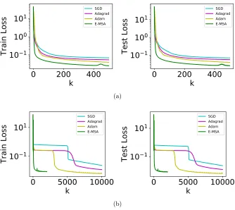
Figure 1: Comparison of E-MSA with gradient-based methods for approximating the sine function with a continuous, 5-dimensional dynamical system. A training and test set of 1000 samples each are used. (a) Loss function vs iterations for a good initialization, where weights are initialized with truncated random normal variables with standard deviation 0.1 and biases are initialized as constants equal to 0.1. We see that E-MSA has good convergence rate per iteration. (b) We use a poor initialization by setting all weights and biases to 0. We observe that gradient descent based methods tend to become stuck whereas E-MSA are better at escaping these slow manifolds, provided thatρ is well chosen (=1.0 in this case).
are not of residual form, but we can nevertheless apply Algorithm 3 with the appropriate
g. We use a total of 10 layers (2 projections, 1 fully-connected and 7 residual layers with
δ = 0.5, i.e T = 3.5). The model is trained with mini-batch sizes of 100 using E-MSA and gradient-descent based methods, namely SGD, Adagrad, and Adam. For E-MSA, we ap-proximately solve the Hamiltonian maximization step using either 10 iterations of L-BFGS. Note that since we have decoupled the layers through the PMP, the L-BFGS step used to maximizeH is tractable since it involves much fewer parameters than directly minimizing
J. Figure 2 compares the performance of E-MSA with the other gradient-descent based methods, where we observe that E-MSA has good performance per-iteration, especially at early stages of training. However, we also show in Figure 3 that the wall-clock performance of our methods are not currently competitive, because the Hamiltonian maximization step is time consuming and the performance gains per iteration is outweighed by the running time. Note that wall-clock times are compared on the CPU for fairness since we did not use a GPU implementation of L-BFGS. As a further test, we train the same model on a different data set, the fashion MNIST data set (Xiao et al., 2017), where we again observe similar phenomena (see Figure 4). Experiments on more complex data sets such as Ima-geNet (Deng et al., 2009) with larger residual networks is a direction of future work. In particular, this may require further improvements to the Hamiltonian maximization step current handled by direct minimization with L-BFGS, which can be significantly slower (on a wall-clock basis) for larger networks and data sets.
6. Discussion and Related Work
0 1 2 3 4 5 6 7 8 910
Epoch
10
1
10
0
Train Loss
SGD Adagrad Adam E-MSA
0 1 2 3 4 5 6 7 8 910
Epoch
10
1
10
0
Test Loss
SGD Adagrad Adam E-MSA
(a)
0 1 2 3 4 5 6 7 8 910
Epoch
0.80
0.85
0.90
0.95
1.00
Train Accuracy
SGD Adagrad Adam E-MSA
0 1 2 3 4 5 6 7 8 910
Epoch
0.80
0.85
0.90
0.95
1.00
Test Accuracy
SGD Adagrad Adam E-MSA
(b)
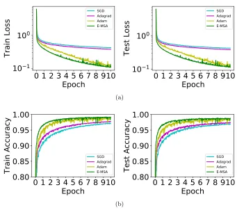
Figure 2: Comparison of E-MSA with gradient-based methods for the residual CNN on the MNIST data set. Mini-batch size of 100 is used so that each epoch of training consists of 550 iterations. (a) Train and test Loss vs epoch. (b) Train and test accuracy vs epoch. For each case, we tuned the associated hyper-parameters on a coarse grid for optimal performance. We observe that per-iteration, E-MSA performs favorably, at least at early times. This shows that if the augmented Hamiltonian can be efficiently maximized, we may obtain good performance.
are very different in behavior compared with gradient-descent based approaches. Again, Lemma 2 ensures that such heuristic global maximization need only be approximate.
0
20
Seconds
10
1
10
0
10
1
Train Loss
SGD Adagrad Adam E-MSA
0
20
Seconds
10
1
10
0
10
1
Test Loss
SGD Adagrad Adam E-MSA
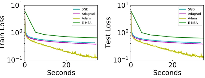
Figure 3: Comparison of E-MSA with gradient-based methods for the residual CNN on the MNIST data set on a wall-clock basis. We observe that currently, the gains per iteration is outweighed by the additional computational costs. Note that we did not use a GPU implementation for the L-BFGS algorithm used to maximize the augmented Hamiltonian, hence the wall-clock time for E-MSA is expected to be improved. Nevertheless, we expect that more efficient Hamiltonian maximization algorithms must be developed for E-MSA to out-perform gradient-based methods in terms of wall-clock efficiency.
different layers, loss functions and models, so specialized algorithms may be designed; (3) The Hamiltonian does not need to be maximized exactly, thus fast heuristic methods (Lee and El-Sharkawi, 2008) or learning (Andrychowicz et al., 2016; Jaderberg et al., 2016; Czar-necki et al., 2017) can potentially be used to perform this. All these are worthy of future exploration in order to make E-MSA truly competitive.
0 1 2 3 4 5 6 7 8 910
Epoch
10
0
Train Loss
SGD Adagrad Adam E-MSA
0 1 2 3 4 5 6 7 8 910
Epoch
10
0
Test Loss
SGD Adagrad Adam E-MSA
(a)
0 1 2 3 4 5 6 7 8 910
Epoch
0.6
0.7
0.8
0.9
Train Accuracy
SGD Adagrad Adam E-MSA
0 1 2 3 4 5 6 7 8 910
Epoch
0.6
0.7
0.8
0.9
Test Accuracy
SGD Adagrad Adam E-MSA
(b)
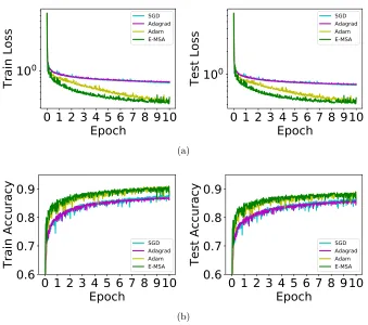
Figure 4: Comparison of E-MSA with gradient-based methods for the residual CNN on the fashion MNIST data set. We use the same network structure and mini-batch sizes as in Figure 2. The hyper-parameters have to be slightly re-tuned. (a) Train and test Loss vs epoch. (b) Train and test accuracy vs epoch. Again, we observe E-MSA performs favorably per-iteration.
PMP, Proposition 3), which then allows us to control errors in the Hamiltonian dynamical equations at every iteration without going into finer mesh-sizes. The regularization terms proportional toρis similar to the heuristic modifications suggested in Lyubushin (1982) by regularizing the distance between θk and θk+1, but we do not have to assume convexity of Θ or that f is Lipschitz inθ.
has been explored in Li et al. (2017) in the form of stochastic optimization. Our current work is also in this flavor, but for neural network models.
In deep learning, there are a few works that share our perspective of deep neural net-works as a discretization of a dynamical system. We note that the connection between the PMP and back-propagation has been pointed out qualitatively in LeCun (1988) and in the development of back-propagation (Bryson, 1975; Baydin et al., 2015), although to the best of our knowledge, this work is the first attempt to translate numerical algorithms for the PMP into training algorithms for deep learning that goes beyond gradient descent. The treatment of machine learning as function approximation via a dynamical system has been presented in E (2017). The recent work of Haber and Ruthotto (2017); Chang et al. (2017) also propose the dynamical systems viewpoint, and the authors used continuous-time tools to address stability issues. In contrast, our work focuses on the optimization aspects cen-tered around the PMP. We also mention other recent approaches to decouple optimization in deep neural networks, such as synthetic gradients (Jaderberg et al., 2016; Czarnecki et al., 2017) and proximal back-propagation (Frerix et al., 2017).
7. Conclusion and Outlook
In this paper, we discuss the viewpoint that deep residual neural networks can be viewed as discretization of a continuous-time dynamical system, and hence supervised deep learning can be regarded as solving an optimal control problem in continuous time. We explore a concrete consequence of this connection, by modifying the classical method of successive approximations for solving optimal control problems (in particular the PMP) into a method for solving a weaker sufficient condition (extended PMP). We prove the convergence of the resulting algorithm (E-MSA) and test it on various benchmark problems, where we observe that the E-MSA algorithm performs favorably on a per-iteration basis, especially at early stages of training, compared with gradient-based approaches such as SGD, Adagrad and Adam.
Acknowledgments
The work of W. E is supported in part by Major Program of NNSFC under grant 91130005, ONR grant N00014-13-1-0338, DOE grants DE-SC0008626 and DE-SC0009248 Q. Li is supported by the Agency for Science, Technology and Research, Singapore.
Appendix A. Function Space Formulation
In this section, we give an alternative, non-rigorous formulation of the supervised learning problem as an optimal control problem on function spaces. This provides an alternative formulation of (continuous-time) deep learning that does not make reference to a specific set of input-outputs, but rather their conditional distributions. The idea is to consider the control of a continuity equation that describes the evolution of probability densities. Hereafter, we proceed formally by assuming all differentiability and integrability conditions are satisfied.
We would like to approximate, using a dynamical systems approach, some target joint probability density ρ(x, y), where x ∈ X ⊂ Rd is a sample input and y ∈ Y is the corre-sponding label. In the case where the labels are deterministically determined by the samples, i.e. there exists F :X → Y such that y=F(x), we would have ρ(x, y) =ρ(x)δ(F(x)−y). Here,ρ(x) is the marginal density ofρ(x, y). In general, we can write ρ(x, y) =ρ(y|x)ρ(x).
As before, the idea is to consider passing the inputs through a dynamical system
˙
Xt=f(t, Xt, θt), X0 =x. (14)
We begin with a guess of a conditional density ρ0(y|x) of y given x. In the deterministic
case, we may set ρ0(y|x) = δ(y−F0(x)) for some F0 : X → Y (this is like the last layer
of the neural network, be it a regressor or a classifier). Note that F0 is potentially very
different fromF, so that ρ0(·|x) is far from our targetρ(·|x).
To improve this approximation, we drive the initial condition by the controllable dy-namical system (14). That is, we define the approximation at time t of ρ(y|x) to be
ρt(y|x) := hρ0(y|·), uti, with ut denoting the probability density of Xt at time t (push-forward distribution ofXtaccording to (14)). It is well-known thatutfollows the continuity equation, or Liouville equation (Gibbs, 2014); or forward Kolmogorov equation in stochastic processes, but with zero noise (Risken, 1996),
d
dtut=−div(f(t,·, θt)ut), u0 =δx, (15)
where divu=P
i∂u/∂xi is the divergence operator and δx(x
0) =δ(x−x0) is a point-mass
atx. We shall assume that ut∈ H ⊂L2(Rd) for some function space H, for all t∈(0, T]. The goal now is to adjust θ∈ U so thatρt(·|x) is close toρ(·|x). To this end, we define a differentiable loss function Φ(ρ1, ρ2) that measures distances between two conditional
as the following optimal control problem:
min θ∈U Ex∼ρ
Φ(ρt(·|x), ρ(·|x)) +
Z T
0
L(θt)dt
,
d
dtut=−div(f(t,·, θt)ut), u0 =δx. (16)
As before, L is a regularizer on the trainable parameters. Now, (16) is an optimal control problem on the function spaceH.
We now write down formally a set of necessary conditions for optimality, in the form of the Pontryagin’s maximum principle, for the present function-space control problem (16). Define the Hamiltonian functional H: [0, T]× H × H ×Θ→R
H(t, u, v, θ) :=−hv,div(f(t,·, θ)u)i −L(θ)
=−
Z
Rd
v(x) d
X
i=1 ∂ ∂xi
(f(t, x, θ)u(x))dx−L(θ).
Then, the Pontryagin’s maximum principle for this system is expected to take the form: let
θ∗ ∈ U be an optimal control, then there exists a co-state processvt∈ H such that
d dtu
∗
t =DvH(t, u∗t, v
∗
t, θ
∗
t), u
∗ 0 =δx,
d dtv
∗
t =−DuH(t, ut∗, v∗t, θt∗), v∗T =−DuΦ(hρ0, u∗Ti, ρ(·|x)) Ex∼ρH(t, u∗t, v
∗
t, θ
∗
t)≥Ex∼ρH(t, u∗t, v
∗
t, θ), θ∈Θ, t∈[0, T],
where D denotes the usual Fr´echet derivative. Note that by definition, we have DvH = −div(f u) and DuH = f · ∇xv. Observe that the co-state v∗ satisfies the (time-reversed) adjoint Liouville’s equation with a specified terminal condition. The PMP for similar func-tional optimal control problems has been studied in, among others, Pogodaev (2016); Roy and Borz (2017), albeit without the expectation over initial density.
In summary, the advantage of this formulation is that we make no explicit reference to the training data or target functions and formulate the entire problem as a control problem on probability densities. Of course, in practice, to implement an MSA-like algorithm, the terminal condition of the co-state will depend on the target joint density, which we can only access through the sampled data. A rigorous analysis of this function space control formulation and its consequences will be explored in future work.
Appendix B. Proof of Lemma 2
First, observe that assumptions (A1)-(A2) in the main text implies that the second deriva-tives off and Φ are bounded byK. Provided thatPtθ is bounded, they also imply that the second derivatives ofH with respect tox andpare bounded when evaluated onXtθ, Ptθ, θt. We first establish the boundedness ofPtθ.
Lemma 6 Assume that (A1)-(A2) hold. Then, there exists a constant K0 > 0 such that for anyθ,
for all t∈[0, T].
Proof Using (7) and setting τ :=T−t, ˜Pτθ :=PTθ−τ we get ˙˜
Pτθ = ˜Pτθ· ∇xf(t, XTθ−τ, T−τ), P˜0θ =−∇Φ(XTθ).
Using (A1)-(A2), we have kPTθk=k∇xΦ(XTθ)k ≤K and k∇xf(t, Xtθ, θt)k2 ≤K. Hence,
kP˙˜τθk ≤KkP˜τθk,
and by Gronwall’s inequality,
kP˜τθk ≤KeKT =:K0.
This proves the claim since it holds for anyτ.
We now prove Lemma 2. The approach here is similar to that employed in Rozonoer (1959).
Proof[Proof of Lemma 2] From (6) and the definition of the Hamiltonian, we have for any
θ∈ U,
I(Xθ, Pθ, θ) :=
Z T
0
Ptθ·X˙tθ−H(t, Xtθ, Ptθ, θt)−L(θt)dt≡0.
DenoteδXt=Xtφ−Xtθ and δPt=Ptφ−Ptθ, then we have
0≡I(Xφ, Pφ, φ)−I(Xθ, Pθ, θ)
=
Z T
0
Ptθ·δX˙t+δPt·X˙tθ+δPt·δX˙tdt
−
Z T
0
H(t, Xtφ, Ptφ, φt)−H(t, Xtθ, Ptθ, θt)dt
−
Z T
0
L(φt)−L(θt)dt. (17)
Now, by integration by parts
Z T
0
Ptθ·δX˙tdt=Ptθ·δXt
T 0 − Z T 0 ˙
Ptθ·δXtdt, (18)
Z T
0
δPt·δX˙tdt=δPt·δXt
T 0 − Z T 0
δP˙t·δXtdt. (19)
Using (6), (7) and (18), we have
Z T
0
Ptθ·δX˙t+δPt·X˙tθdt
=Ptθ·δXt
T 0 + Z T 0
f(t, Xtθ;θt)·δP +∇xH(t, Xtθ, Ptθ, θt)·δX
dt
=Ptθ·δXt
T 0 + Z T 0
∇zH(t, Ztθ, θt)·δZ
where in the last line we defined Zθ := (Xθ, Pθ). Similarly, from (19) we get
Z T
0
δPt·δX˙tdt= 1 2
Z T
0
δPt·δX˙tdt+ 1 2
Z T
0
δPt·δX˙tdt
=1
2δPt·δXt
T 0 + 1 2 Z T 0
[∇zH(t, Ztφ, φt)− ∇zH(t, Ztθ, θt)]·δZt
dt
=1
2δPt·δXt
T 0 + 1 2 Z T 0
[∇zH(t, Ztθ, φt)− ∇zH(t, Ztθ, θt)]·δZtdt
+ 1 2
Z T
0
δZt· ∇2zH(t, Ztθ+r1(t)δZt, φt)·δZtdt. (21) where we have used Taylor’s theorem in the last step with r1(t) ∈ [0,1]. We now rewrite
the boundary terms. Since δX0 = 0, we have
(Ptθ+1
2δPt)·δXt
T
0 = (P
θ T +
1
2δPT)·δXT
=− ∇Φ(XTθ)·δXT − 1
2(∇Φ(X φ
T)− ∇Φ(X θ
T))·δXT
=− ∇Φ(XTθ)·δXT − 1
2δXT · ∇
2Φ(Xθ
T +r2δXT)·δXT =−(Φ(XTφ)−Φ(XTθ))−1
2δXT ·(∇
2Φ(Xθ
T +r2δXT) +∇2Φ(XTθ +r3δXT))·δXT, (22) for somer2, r3 ∈[0,1]. Lastly, for each t∈[0, T] we have
H(t, Ztφ, φt)−H(t, Ztθ, θt) =H(t, Ztθ, φt)−H(t, Ztθ, θt)
+∇zH(t, Ztθ, φt)·δZt
+1
2δZt· ∇
2
zH(t, Ztθ+r4(t)δZt, φt)·δZt, (23) wherer4(t)∈[0,1].
Substituting (20), (21), (22), (23) into (17), we obtain
Φ(XTφ) +
Z T
0
L(φt)
−
Φ(XTθ) +
Z T
0 L(θt)
=1
2δXT ·(∇
2Φ(Xθ
T +r2δXT) +∇2Φ(XTθ +r3δXT))·δXT −
Z T
0
∆Hφ,θ(t)dt
+ 1 2
Z T
0
(∇zH(t, Ztθ, φt)− ∇zH(t, Ztθ, θt))·δZtdt
+ 1 2
Z T
0
δZt·[∇2zH(t, Ztθ+r1(t)δZt, φt)− ∇2zH(t, Ztθ+r4(t)δZt, φt)]·δZt
The left hand side is simplyJ(φ)−J(θ), and so it remains to estimate the right hand side terms. First, let us estimate δX and δP. By definition,
δX˙t=f(t, Xtφ, φt)−f(t, Xtθ, θt).
Integrating, we get
δXt=
Z t
0
f(t, Xsφ, φs)−f(t, Xsθ, θs)ds,
and so
kδXtk ≤
Z t
0
kf(t, Xsφ, φs)−f(t, Xsθ, θs)kds
≤
Z t
0
kf(t, Xsφ, φs)−f(t, Xsθ, φs)kds
+
Z t
0
kf(t, Xsθ, φs)−f(t, Xsθ, θs)kds
≤
Z T
0
kf(t, Xsθ, φs)−f(t, Xsθ, θs)kds
+K
Z t
0
kδXskdt. (25)
By Gronwall’s inequality, we have
kδXtk ≤eKT
Z T
0
kf(t, Xsθ, φs)−f(t, Xsθ, θs)kds. (26)
To estimateδP, we use the same substitution as in Lemma 6 withτ =T−tand ˜·τ =·T−t. We get
δP˜τ =δP˜0+
Z τ
0
∇xH(t,X˜sφ,P˜sφ,φ˜s)− ∇xH(t,X˜sθ,P˜sθ,θ˜s)ds,
and hence using Lemma 6 and assumptions (A1)-(A2),
kδP˜τk ≤kδP˜0k+
Z τ
0
k∇xH(t,X˜sφ,P˜sφ,φ˜s)− ∇xH(t,X˜sθ,P˜sθ,θ˜s)kds
≤KkδXTk+KK0
Z T
0
kδXskds+K
Z τ
0
kδP˜skds
+
Z T
0
k∇xH(t, Xsθ, Psθ, φs)− ∇xH(t, Xsθ, Psθ, θs)kds
≤eKTK(kδXTk+K0
Z T
0
kδXskds)
+eKT
Z T
0
Using estimate (26), we obtain
kδPtk ≤e2KTK(1 +K0T)
Z T
0
kf(t, Xsθ, φs)−f(t, Xsθ, θs)kds
+eKT
Z T
0
k∇xH(t, Xsθ, Psθ, φs)− ∇xH(t, Xsθ, Psθ, θs)kds. (28)
Now, we substitute estimates (26) and (28) into (24) and rename constants for simplicity. Note that by assumptions (A1)-(A2) and Lemma 6, all the second derivative terms are bounded element-wise by some constantK00. Hence, we have |δZt·A·δZt| ≤K00kδZk2 for each A being a second derivative matrix. Thus we obtain
J(φ)−J(θ)≤ −
Z T
0
∆Hφ,θ(t)dt
+1 2K
00kδX
Tk2 +K00
Z T
0
(kδXtk2+kδPtk2)dt
+1 2
Z T
0
kδXtkkf(t, Xtθ, φt)−f(t, Xtθ, θt)kdt
+1 2
Z T
0
kδPtkk∇xH(t, Xtθ, Ptθ, φt)− ∇xH(t, Xtθ, Ptθ, θt)kdt
≤ −
Z T
0
∆Hφ,θ(t)dt
+C
Z T
0
kf(t, Xtθ, φt)−f(t, Xtθ, θt)kdt
2
+C
Z T
0
k∇xH(t, Xtθ, Ptθ, φt)− ∇xH(t, Xtθ, Ptθ, θt)k2dt
2
(29)
≤ −
Z T
0
∆Hφ,θ(t)dt
+C
Z T
0
kf(t, Xtθ, φt)−f(t, Xtθ, θt)k2dt
+C
Z T
0
k∇xH(t, Xtθ, Ptθ, φt)− ∇xH(t, Xtθ, Ptθ, θt)k2dt.
Remark 7 For applications, the global Lipschitz condition (A2) w.r.t. x on f may be restrictive. Note that this can be replaced by a local Lipschitz condition if we can show that
Xt, t∈ [0, T] is bounded for all θ ∈ U. This is true if the parameter space Θ is bounded,
References
Vladimir V Aleksandrov. On the accumulation of perturbations in the linear systems with two coordinates. Vestnik MGU, 3, 1968.
Marcin Andrychowicz, Misha Denil, Sergio Gomez, Matthew W Hoffman, David Pfau, Tom Schaul, and Nando de Freitas. Learning to learn by gradient descent by gradient descent. In Advances in Neural Information Processing Systems, pages 3981–3989, 2016.
Michael Athans and Peter L Falb. Optimal control: an introduction to the theory and its applications. Courier Corporation, 2013.
Atilim G Baydin, Barak A Pearlmutter, Alexey A Radul, and Jeffrey M Siskind. Automatic differentiation in machine learning: a survey. arXiv preprint arXiv:1502.05767, 2015.
Mokhtar S Bazaraa, Hanif D Sherali, and Chitharanjan M Shetty. Nonlinear programming: theory and algorithms. John Wiley & Sons, 2013.
Richard Bellman. Dynamic programming. Courier Corporation, 2013.
Yoshua Bengio. Learning deep architectures for AI. Foundations and trends in Machine Learning, 2(1):1–127, 2009.
Dimitri P Bertsekas.Dynamic programming and optimal control, volume 1. Athena scientific Belmont, MA, 1995.
Dimitri P Bertsekas. Nonlinear programming. Athena scientific Belmont, 1999.
John T Betts. Survey of numerical methods for trajectory optimization.Journal of Guidance control and dynamics, 21(2):193–207, 1998.
Vladimir Grigor’evich Boltyanskii, Revaz Valer’yanovich Gamkrelidze, and Lev Semenovich Pontryagin. The theory of optimal processes. i. the maximum principle. Technical report, TRW SPACE TECHNOLOGY LABS LOS ANGELES CALIF, 1960.
L´eon Bottou. Large-scale machine learning with stochastic gradient descent. InProceedings of COMPSTAT’2010, pages 177–186. Springer, 2010.
Alberto Bressan and Benedetto Piccoli. Introduction to mathematical control theory. AIMS series on applied mathematics, Philadelphia, 2007.
Arthur Earl Bryson. Applied optimal control: optimization, estimation and control. CRC Press, 1975.
Anatolii B Butkovsky. Necessary and sufficient optimality conditions for sampled-data control systems. Avtomat. i Telemekh, 24(8):1056–1064, 1963.
Felix L Chernousko and Alexey A Lyubushin. Method of successive approximations for solution of optimal control problems. Optimal Control Applications and Methods, 3(2): 101–114, 1982.
Francis Clarke. The maximum principle in optimal control, then and now. Control and Cybernetics, 34(3):709, 2005.
Matthieu Courbariaux, Yoshua Bengio, and Jean-Pierre David. Binaryconnect: Training deep neural networks with binary weights during propagations. In Advances in Neural Information Processing Systems, pages 3123–3131, 2015.
Matthieu Courbariaux, Itay Hubara, Daniel Soudry, Ran El-Yaniv, and Yoshua Bengio. Binarized neural networks: Training deep neural networks with weights and activations constrained to + 1 or - 1. arXiv preprint arXiv:1602.02830, 2016.
Wojciech M Czarnecki, Grzegorz ´Swirszcz, Max Jaderberg, Simon Osindero, Oriol Vinyals, and Koray Kavukcuoglu. Understanding synthetic gradients and decoupled neural inter-faces. arXiv preprint arXiv:1703.00522, 2017.
J. Deng, W. Dong, R. Socher, L.-J. Li, K. Li, and L. Fei-Fei. ImageNet: A Large-Scale Hierarchical Image Database. InCVPR09, 2009.
John Duchi, Elad Hazan, and Yoram Singer. Adaptive subgradient methods for online learning and stochastic optimization. Journal of Machine Learning Research, 12(Jul): 2121–2159, 2011.
Weinan E. A proposal on machine learning via dynamical systems. Communications in Mathematics and Statistics, 5(1):1–11, 2017.
Thomas Frerix, Thomas M¨ollenhoff, Michael Moeller, and Daniel Cremers. Proximal back-propagation. arXiv preprint arXiv:1706.04638, 2017.
J Willard Gibbs.Elementary principles in statistical mechanics. Courier Corporation, 2014.
Ian Goodfellow, Yoshua Bengio, and Aaron Courville. Deep learning. MIT press, 2016.
Eldad Haber and Lars Ruthotto. Stable architectures for deep neural networks. arXiv preprint arXiv:1705.03341, 2017.
Richard HR Hahnloser, Rahul Sarpeshkar, Misha A Mahowald, Rodney J Douglas, and H Sebastian Seung. Digital selection and analogue amplification coexist in a cortex-inspired silicon circuit. Nature, 405(6789):947, 2000.
Hubert Halkin. A maximum principle of the pontryagin type for systems described by nonlinear difference equations. SIAM Journal on control, 4(1):90–111, 1966.
Magnus R Hestenes. Multiplier and gradient methods. Journal of optimization theory and applications, 4(5):303–320, 1969.
R Jackson and F Horn. On discrete analogues of pontryagin’s maximum principle. Inter-national Journal of Control, 1(4):389–395, 1965.
Max Jaderberg, Wojciech M Czarnecki, Simon Osindero, Oriol Vinyals, Alex Graves, and Koray Kavukcuoglu. Decoupled neural interfaces using synthetic gradients.arXiv preprint arXiv:1608.05343, 2016.
Robert I Jennrich. Asymptotic properties of non-linear least squares estimators.The Annals of Mathematical Statistics, 40(2):633–643, 1969.
Rie Johnson and Tong Zhang. Accelerating stochastic gradient descent using predictive variance reduction. In Advances in neural information processing systems, pages 315– 323, 2013.
Henry J Kelley. Gradient theory of optimal flight paths.Ars Journal, 30(10):947–954, 1960.
Diederik Kingma and Jimmy Ba. Adam: A method for stochastic optimization. arXiv preprint arXiv:1412.6980, 2014.
Ivan A Krylov and Felix L Chernousko. On the method of successive approximations for solution of optimal control problems. J. Comp. Mathem. and Mathematical Physics, 2 (6), 1962.
Yann LeCun. A theoretical framework for back-propagation. InThe Connectionist Models Summer School, volume 1, pages 21–28, 1988.
Yann LeCun. The MNIST database of handwritten digits. http://yann. lecun. com/exdb/mnist/, 1998.
Yann LeCun and Yoshua Bengio. Convolutional networks for images, speech, and time series. The handbook of brain theory and neural networks, 3361(10):1995, 1995.
Yann LeCun, L´eon Bottou, Yoshua Bengio, and Patrick Haffner. Gradient-based learning applied to document recognition. Proceedings of the IEEE, 86(11):2278–2324, 1998.
Yann LeCun, Yoshua Bengio, and Geoffrey Hinton. Deep learning. Nature, 521(7553): 436–444, 2015.
Kwang Y Lee and Mohamed A El-Sharkawi. Modern heuristic optimization techniques: theory and applications to power systems, volume 39. John Wiley & Sons, 2008.
Qianxiao Li, Cheng Tai, and Weinan E. Stochastic modified equations and adaptive stochas-tic gradient algorithms. In International Conference on Machine Learning, pages 2101– 2110, 2017.
Dong C Liu and Jorge Nocedal. On the limited memory BFGS method for large scale optimization. Mathematical programming, 45(1):503–528, 1989.
Alexey A Lyubushin. Modifications of the method of successive approximations for solving optimal control problems. USSR Computational Mathematics and Mathematical Physics, 22(1):29–34, 1982.
Zbigniew Nahorski, Hans F Ravn, and Ren´e Victor Valqui Vidal. The discrete-time maxi-mum principle: a survey and some new results. International Journal of Control, 40(3): 533–554, 1984.
Nikolay Pogodaev. Optimal control of continuity equations. Nonlinear Differential Equa-tions and ApplicaEqua-tions, 23(2):21, 2016.
Lev S Pontryagin. Mathematical theory of optimal processes. CRC Press, 1987.
Anil V Rao. A survey of numerical methods for optimal control. Advances in the Astro-nautical Sciences, 135(1):497–528, 2009.
Hannes Risken. Fokker-planck equation. In The Fokker-Planck Equation, pages 63–95. Springer, 1996.
Herbert Robbins and Sutton Monro. A stochastic approximation method. The annals of mathematical statistics, pages 400–407, 1951.
Sanford M Roberts and Jerome S Shipman. Two-point boundary value problems: shooting methods. SIAM Rev., 16(2):265266, 1972.
Souvik Roy and Alfio Borz. Numerical investigation of a class of liouville control problems.
J Sci Comput, 73:178, 2017.
Lev I Rozonoer. The maximum principle of L.S. Pontryagin in optimal-system theory.
Automation and Remote Control, 20(10):11, 1959.
J¨urgen Schmidhuber. Deep learning in neural networks: An overview. Neural networks, 61: 85–117, 2015.
Ilya Sutskever, James Martens, George Dahl, and Geoffrey Hinton. On the importance of initialization and momentum in deep learning. In International conference on machine learning, pages 1139–1147, 2013.
Gavin Taylor, Ryan Burmeister, Zheng Xu, Bharat Singh, Ankit Patel, and Tom Gold-stein. Training neural networks without gradients: A scalable ADMM approach. In
International Conference on Machine Learning, pages 2722–2731, 2016.
Han Xiao, Kashif Rasul, and Roland Vollgraf. Fashion-MNIST: a novel image dataset for benchmarking machine learning algorithms. arXiv preprint arXiv:1708.07747, 2017.