Differentially Private Data Releasing for Smooth Queries
Ziteng Wang [email protected]
Key Laboratory of Machine Perception (MOE), School of EECS Peking University
Beijing, 100871, China
Chi Jin [email protected]
Department of Computer Science University of California
Berkeley, CA 94720-1776, USA
Kai Fan [email protected]
Computational Biology & Bioinformactics Duke University
Durham, NC 27708, USA
Jiaqi Zhang [email protected]
Key Laboratory of Machine Perception (MOE), School of EECS Peking University
Beijing, 100871, China
Junliang Huang [email protected]
School of Mathematical Sciences Peking University
Beijing, 100871, China
Yiqiao Zhong [email protected]
School of Mathematical Sciences Peking University
Beijing, 100871, China
Liwei Wang [email protected]
Key Laboratory of Machine Perception (MOE), School of EECS Peking University
Beijing, 100871, China
Editor:Sanjoy Dasgupta
Abstract
In the past few years, differential privacy has become a standard concept in the area of pri-vacy. One of the most important problems in this field is to answer queries while preserving differential privacy. In spite of extensive studies, most existing work on differentially pri-vate query answering assumes the data arediscrete (i.e., in{0,1}d) and focuses on queries induced byBooleanfunctions. In real applications however,continuous data are at least as common as binary data. Thus, in this work we explore a less studied topic, namely, differen-tial privately query answering for continuous data with continuous function. As a first step
towards the continuous case, we study a natural class of linear queries on continuous data which we refer to assmooth queries. A linear query is said to beK-smooth if it is specified by a function defined on [−1,1]d whose partial derivatives up to orderK are all bounded. We develop two -differentially private mechanisms which are able to answer all smooth queries. The first mechanism outputs a summary of the database and can then give answers to the queries. The second mechanism is an improvement of the first one and it outputs a synthetic database. The two mechanisms both achieve an accuracy ofO(n−2dK+K/). Here
we assume that the dimension d is a constant. It turns out that even in this parameter setting (which is almost trivial in the discrete case), using existing discrete mechanisms to answer the smooth queries is difficult and requires more noise. Our mechanisms are based onL∞-approximation of (transformed) smooth functions by low-degree even
trigonomet-ric polynomials with uniformly bounded coefficients. We also develop practically efficient variants of the mechanisms with promising experimental results.1
Keywords: differential privacy, smooth queries, synthetic dataset
1. Introduction
Statistical analysis and machine learning are often conducted on data sets containing sen-sitive information, such as medical records, commercial data, etc. The benefit of mining from such data is tremendous. But when releasing sensitive data, one must take privacy issue into consideration, and has to accept a tradeoff between the accuracy and the amount of privacy loss of the individuals in the database.
In this paper, we consider differential privacy (Dwork et al., 2006), which has become a standard concept in the area of privacy. Roughly speaking, a mechanism which releases information about some database is said to preserve differential privacy, if the change of a single database element does not affect the probability distribution of the output signif-icantly. Differential privacy provides strong guarantees against attacks. It ensures that the risk of information leakage for any individual who submits her information to the database is very small, in the sense that an adversary can discover almost nothing new from the database that contains one individual’s information compared with that from the database without that individual’s information. Recently there have been extensive studies of machine learning, statistical estimation, and data mining under the differential privacy framework (Wasserman and Zhou, 2010; Chaudhuri et al., 2011; Lei, 2011; Kifer and Lin, 2010; Chaudhuri et al., 2012; Williams and McSherry, 2010; Jain et al., 2012; Chaudhuri and Hsu, 2011).
Accurately answering statistical queries is a well studied problem in differential privacy. A simple and efficient method is the Laplace mechanism (Dwork et al., 2006), which adds Laplace noise to the true answers. Laplace mechanism is especially useful for queries with low sensitivity, which is the maximal difference of the query values of two databases that are different in only one item. A typical class of queries that has low sensitivity is linear queries, whose sensitivity isO(1/n), wheren is the size of the database.
The Laplace mechanism has a limitation. It can answer at most O(n2) queries. If the number of queries is substantially larger thann2, Laplace mechanism is not able to provide differentially private answers with nontrivial accuracy. Considering that potentially there are many users and each user may submit a set of queries, limiting the number of total
queries to be smaller than n2 is too restricted in some situations. A remarkable result due to Blum, Ligett and Roth (Blum et al., 2008) (will be referred to as BLR in this paper) shows that: information theoretically it is possible for a mechanism to answer far more than n2
linear queries while preserving differential privacy and nontrivial accuracy simultaneously. There is a series of works (Dwork et al., 2009, 2010; Roth and Roughgarden, 2010; Hardt and Rothblum, 2010) improving the result of (Blum et al., 2008). All these mechanisms are very powerful in the sense that they can answer general and adversely chosen queries. On the other hand, even the fastest algorithms for query answering (Hardt and Rothblum, 2010; Hardt et al., 2012a) run in time linear in the size of the data universe. Often the size of the data universe is much larger than that of the database, so these mechanisms are inefficient. Recently, Ullman (2013) shows that there is no polynomial time algorithm that can answern2+o(1) general linear queries while preserving privacy and accuracy (assuming the existence of one-way function).
Recently, there are growing interests in studying differentially private mechanisms for restricted classes of queries, in particular queries useful in applications. One class of queries that attracts a lot of attentions are the k-way conjunctions. The data universe for this problem is{0,1}d. Thus each individual record hasdbinary attributes. A k-way
conjunc-tion query is specified bykfeatures. The query asks what fraction of the individual records in the database has all thesekfeatures being 1. A series of works attack this problem using several different techniques (Barak et al., 2007; Gupta et al., 2011; Cheraghchi et al., 2012; Hardt et al., 2012b; Thaler et al., 2012) . They proposed elegant mechanisms which run in time poly(n) whenkis a constant. Another class of queries that yields efficient mechanisms is the class of sparse query. A query is m-sparse if it takes non-zero values on at most m
elements in the data universe. Blum and Roth (2013) developed mechanisms which are efficient whenm= poly(n).
The above differentially private mechanisms can also be categorized into two classes according to the output of the algorithm. The first class of algorithms output answers to the queries. The second class of algorithms output synthetic databases instead; the answers of the queries can then be simply computed from the synthetic database. The Laplace mechanism belongs to the first class. BLR and the offline version of the Private Multiplicative Weight updating (PMW) mechanism (Hardt and Rothblum, 2010; Hardt et al., 2012a) output synthetic database. From a practical point of view, the synthetic dataset output is appealing. In fact, before the notion of differential privacy was proposed, almost all practical techniques developed to preserve privacy against certain types of attacks output a synthetic dataset by modifying the raw dataset (please see the survey Aggarwal and Yu 2008 and the references therein).
Among the studies of differentially private query answering, most existing works focus on binary data and queries induced by Boolean functions2. In real applications however,
continuous data are at least as common as binary data; and one has to use continuous functions in this scenario instead of Boolean functions. In this paper, we explore this relatively less studied topic, i.e., differentially private query answering with continuous
functions on continuous data. We assume that 1) the data universe is X = [−1,1]d; 2) a linear queryqf is induced by a continuous function f :X →R.
As will be clear soon, answering general linear queries in the continuous setting is con-siderably more difficult than that in the binary case. Therefore we will focus our analysis on a restricted class of linear queries. The first question is: which subclass of linear queries is commonly used in practice? LetD={x1, . . . , xn} (xi ∈[−1,1]d) be a database consisting
of continuous data. A linear query qf on D is defined as qf(D) := n1Px∈Df(x), where
f : [−1,1]d→
Ris a continuous function. Thus, to find out a natural class of linear queries,
one only needs to find out a natural class of continuous functions.
The set of continuous functions considered in this paper is the set of smooth queries. We say a functionf : [−1,1]d→RisK-smooth, if all the partial derivatives off up to the
Kth order are bounded. We say a linear queryqf isK-smooth iff is aK-smooth function.
We believe smooth function is one of the most natural and useful classes of continuous functions; and therefore the set of smooth queries is a natural class of linear queries worth studying. Our aim is to answer all smooth queries while preserving differential privacy and accuracy. See also section 4.2 for an explanation of why answering all smooth queries is useful for differentially private machine learning. As a first step towards differential privacy for continuous query, we study in this work the case where the dimensiondof the data universe [−1,1]d is a constant. It turns out that the smooth query problem is very challenging even ford=O(1) which is almost trivial in the discrete case (see below).
We develop two mechanisms for the smooth query. The two mechanisms both achieve
accuracy ofO n12dK+K
/forall K-smooth queries. If the order of smoothnessK is large compared to the dimensiond, then the errors of the mechanisms are close ton−1.
To be more concrete, the former mechanism outputs a summary of the database. To ob-tain an answer of a smooth query, the user runs a public evaluation procedure which conob-tains no information of the database. Outputting the summary has running timeOn1+2d+dK
,
and the evaluation procedure for answering a query runs in time ˜O(n
d+2+ 2d K
2d+K ). It can be
seen that ifK is large compared tod, then the mechanism runs in almost linear time. For our second mechanism which outputs synthetic database, the running time is O(n34dKd+2+5Kd),
polynomial in the size of the database. Theoretically, the second mechanism is far less effi-cient as the first one. This is reasonable since outputting synthetic database is much harder than outputting answers. We then develop practically efficient variants of this mechanism.
As a comparison, we will consider how to apply existing mechanisms (e.g., PMW, BLR) to solve the smooth query problem. As our goal is to answer all smooth queries while preserving privacy and accuracy, and because there are infinitely manyK-smooth functions, one has to discretize the set of smooth functions before using any existing mechanism. It is not clear how to efficiently discretize this set of queries. More importantly, we show that even if one can discretize this query set in an optimal way, there is a lower bound for the number of discretized queries of this set. The lower bound is exponential in 1/α, where α
The mechanisms proposed in this paper are based on L∞-approximation and is
mo-tivated by Thaler et al. (2012), which considers approximation of k-way conjunctions by low degree polynomials. Our basic idea is to approximate the whole query class by linear combination of a small set of basis functions. The main technical difficulty lies in that in order that the approximation induces an efficient and differentially private mechanism, all the linear coefficients of the basis functions must be small. To guarantee this, we first trans-form the query function. Then by using even trigonometric polynomials as basis functions we prove a constant upper bound for the linear coefficients. It is worth pointing out that to guarantee accuracy, we must considerL∞-approximation. It is completely different from
L2-approximation, which is simply Fourier analysis when using trigonometric polynomial
as basis. Another difficulty for the first mechanism is how to efficiently compute the linear coefficients. It turns out that the smoothness of the functions allows us to use an efficient numerical method to compute the coefficients to a precision so that the accuracy of the mechanism is not affected significantly.
We also point out that the basis functions described above have some relation to conjunc-tions. In fact, conjunctions can also be viewed as smooth functions as they are multilinear polynomials. Conjunctions form a small subset of smooth functions. Moreover, the set of conjunctions is also a strict subset of the basis function used in our mechanism. If we re-strict to conjunctions, our algorithm essentially reduces to Laplace mechanism (see Section 3.2.2 for details). But different to all existing works dealing with conjunctions, our aim here is to answer all smooth queries while preserving privacy and accuracy.
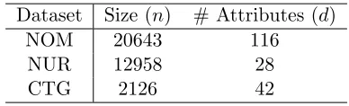
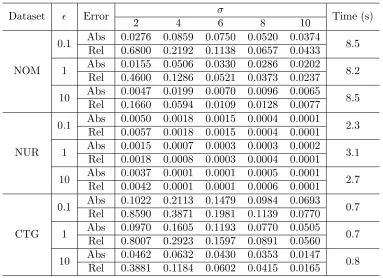
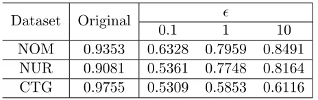
Finally we conduct experiments on the efficient variant of the mechanism which outputs synthetic database as it may be more useful in practice. Experimental results demonstrate that the algorithm achieves good accuracy and are practically efficient on datasets of various sizes and of a number of attributes.
This work is a small step towards an understanding of smooth queries. Our mechanisms have obvious limitations: The performances decrease exponentially with respect to the data dimension d. Thus the algorithms cannot handle the case in which d is a super constant. The experimental results also demonstrate that our mechanisms work well mostly whend
is no more than a few hundred. Studying the general case d=ω(1) is our future work. The rest of the paper is organized as follows. Section 2 gives the background and all the definitions. In Section 3, we propose the query-answering mechanism. In Section 4, we give the mechanism which is able to output synthetic database. In Section 5, we develop a practical variant of the second mechanism and conduct experiments to evaluate its performance. Finally, we conclude in Section 6.
2. Preliminaries
Let D be a database containing n data points in the data universe X. In this paper, we consider the case that X ⊂ Rd whered is a constant. Typically, we assume that the data
universe X = [−1,1]d. Two databases Dand D0 are called neighbors if|D|=|D0|=n and they differ in exactly one data point. The following is the formal definition of differential privacy.
for all pairs of neighbor databases D, D0, the following holds:
P(M(D)∈S)≤P(M(D0)∈S)·e+δ,
where the probability is taken over the randomness of the M. If M preserves (,0) -differential privacy, we say M is-differentially private.
We considerlinear queries. Each linear queryqf is specified by a functionf which maps
the data universe [−1,1]dtoR. qf is defined as
qf(D) :=
1
|D|
X
x∈D
f(x).
Let Qbe a set of queries. The accuracy of a mechanism with respect toQis defined as follows.
Definition 2 ((α, β)-accuracy) Let Q be a set of queries. A mechanism M is said to have (α, β)-accuracy for size n databases with respect to Q, if for every database D with
|D|=n the following holds
P(∃q∈Q, |M(D, q)−q(D)| ≥α)≤β,
where M(D, q) is the answer to q given by M, and the probability is over the internal randomness of the mechanism M.
We will make use of the Laplace mechanism (Dwork et al., 2006) in our algorithm. Laplace mechanism adds Laplace noise to the output. We denote by Lap(σ) the random variable distributed according to the Laplace distribution with parameterσ, whose density function is 2σ1 exp(−|x|/σ).
Next, we formally define smooth queries, which is a special class of linear queries. Since each linear query qf is specified by a function f, a set of queries QF can be specified by
a set of functions F. Remember that each f ∈ F maps [−1,1]d to R. For any point x= (x1, . . . , xd)∈[−1,1]d, if k= (k1, . . . , kd) is ad-tuple of nonnegative integers, then we
define
Dk:=Dk1
1 · · ·D kd d :=
∂k1
∂xk1
1
· · · ∂
kd
∂xkd d
.
Let |k|:=k1+. . .+kd. Define theK-norm as
kfkK := sup
|k|≤K
sup x∈[−1,1]d
|Dkf(x)|.
We will study the set CBK which contains all smooth functions whose derivatives up to order K have ∞-norm upper bounded by a constant B >0. Formally,
CBK :={f : kfkK ≤B}.
The set of queries specified byCK
B, denoted as QCK
B, is our focus. Smooth functions have
1999; Smola et al., 1998; Wang, 2011). See Section 4.2 for examples of smooth functions and its relation to differentially private machine learning.
In this work we will frequently use trigonometric polynomials. For the univariate case, a function p(θ) is called a trigonometric polynomial of degree m if
p(θ) =a0+ m
X
r=1
(arcosrθ+brsinrθ),
wherear, brare constants. Ifp(θ) is an even function, we say that it is an even trigonometric
polynomial, and
p(θ) =a0+ m
X
r=1
arcosrθ.
For the multivariate case, if
p(θ1, . . . , θd) =
X
r=(r1,...,rd)
arcos(r1θ1). . .cos(rdθd),
thenp is said to be an even trigonometric polynomial (with respect to each variable), and the degree of θi is maxi≤d{ri}.
3. The First Mechanism: Query Answering
In this section we propose our first mechanism which outputs answers to the queries. Our second mechanism which is able to output synthetic database will be given in the next section.
3.1 Mechanism and Main Results
The following theorem is our first main result. It says that if the query class is specified by smooth functions, then there is an efficient mechanism for query answering which preserves
-differential privacy and good accuracy. The mechanism consists of two parts: One for outputting a summary of the database, the other for answering a query. The two parts are described in Algorithm 1 and Algorithm 2 respectively. The second part of the mechanism contains no private information of the database.
Theorem 3 Let the query set be
QCK
B :={qf =
1
n
X
x∈D
f(x) : f ∈CBK},
where K ∈N andB >0 are constants. Let the data universe be [−1,1]d, where d∈N is a constant. Then the mechanism M given in Algorithm 1 and Algorithm 2 satisfies that for any >0, the followings hold:
Algorithm 1 Outputting the summary
Notations: Td
t :={0,1, . . . , t−1}d, x:= (x1,· · ·, xd), θi(x) := arccos(xi). Parameters: Privacy parameters, δ >0, Failure probabilityβ >0,
Smoothness orderK ∈N.
Input: Database D∈ [−1,1]dn
Output: Atd-dimensional vector as the summary ˆb.
1: Sett=dn2d+1Ke.
2: for all r= (r1, . . . , rd)∈ Ttd do 3: br ← n1
P
x∈Dcos (r1θ1(x)). . .cos (rdθd(x)) 4: ˆbr ←br+ Lap
td n
5: end for
6: bˆ ←(ˆbr)krk∞≤t−1 (ˆb is at
d dimensional vector)
7: return: bˆ
Algorithm 2 Answering a query
Input: A queryqf, wheref : [−1,1]d→Rand f ∈CBK,
Summary ˆb returned by Algorithm 1
Output: Approximate answer toqf(D). 1: Sett=dn2d+1Ke.
2: Letgf(θ) =f(cos(θ1), . . . ,cos(θd)), θ= (θ1, . . . , θd)∈[−π, π]d.
3: Compute the a trigonometric polynomial approximationpt(θ) ofgf(θ), where
pt(θ) =Pr=(r1,...,rd),krk∞≤t−1crcos(r1θ1). . .cos(rdθd). (see Section 3.3 for details) 4: c←(cr)krk∞≤t−1 (c is at
d dimensional vector)
5: return: c·bˆ
2) For anyβ ≥10·e−15(n d 2d+K)
the mechanism is(α, β)-accurate, whereα =On−2dK+K/
, and the hidden constant depends only on d, K and B.
3) The running time for M to output the summary isO(n32dd++KK).
4) The running time for M to answer a query isO(n
d+2+ 2d K
2d+K ·polylog(n)).
The proof of Theorem 3 is essentially based on Theorem 4 given below. The detailed proof of Theorem 3 is given in the Section 3.4.
To have a better idea of how the performances depend on the order of smoothness, let us consider three cases. The first case isK = 1, i.e., the query functions only have the first order derivatives. Another extreme case isK d, and we assume d/K=0 1. We also
consider a case in the middle by assuming K = 2d. Table 1 gives simplified upper bounds for the error and running time in these cases. We have the following observations:
1) The accuracyαimproves dramatically from roughly O(n−21d) to nearlyO(n−1) asK
Order of smoothness Accuracyα Running Time: Running Time: Outputting summary Answering a query
K = 1 O(n−2d1+1) O(n32) O˜(n 3 2+
1 4d+2)
K = 2d O(n−12) O(n 5
4) O˜(n 1 4+
3/4 d ) d
K =0 1 O(n
−(1−20)) O(n1+0) O˜(n0(1+3d)) Table 1: Performance vs. Order of Smoothness for Query Answering
2) The running time for outputting the summary does not change too much, because reading through the database requires Ω(n) time.
3) The running time for answering a query reduces significantly from roughly O(n3/2) to nearlyO(n0) asK getting large. When K = 2d, it is approximately n1/4 if dis not too small.
Conceptually our mechanism is simple. First, by change of variables we have
gf(θ1, . . . , θd) =f(cosθ1, . . . ,cosθd).
It also transforms the data universe from [−1,1]d to [−π, π]d. Note that for each variable
θi, gf is an even function. To compute the summary, the mechanism just gives noisy
answers to queries specified by even trigonometric monomials cos(r1θ1). . .cos(rdθd). For
each trigonometric monomial, the highest degree of any variable is max1≤i≤dri ≤ t =
O(n2d+1K). The summary is anO(n d
2d+K)-dimensional vector. To answer a query specified
by a smooth functionf, the mechanism computes a trigonometric polynomial approximation ofgf. The answer to the queryqf is a linear combination of the summary by the coefficients
of the approximation trigonometric polynomial.
Our algorithm is anL∞-approximation based mechanism, which is motivated by Thaler
et al. (2012). An approximation based mechanism relies on three conditions:
1) There exists a small set of basis functions such that every query function can be well approximated by a linear combination of them.
2) All the linear coefficients are small.
3) The whole set of the linear coefficients can be computed efficiently.
If these conditions hold, then the mechanism just outputs noisy answers to the set of queries specified by the basis functions as the summary. When answering a query, the mech-anism computes the coefficients with which the linear combination of the basis functions approximate the query function. The answer to the query is sidiscretizationmply the inner product of the coefficients and the summary vector.
Theorem 4 Let γ >0. For everyf ∈CBK defined on [−1,1]d, let
gf(θ1, . . . , θd) =f(cosθ1, . . . ,cosθd), θi ∈[−π, π].
Then, there is an even trigonometric polynomial p whose degree of each variable is t(γ) =
1 γ
1/K :
p(θ1, . . . , θd) =
X
0≤r1,...,rd<t(γ)
cr1,...,rdcos(r1θ1). . .cos(rdθd),
such that
1) kgf−pk∞≤γ.
2) All the linear coefficients cr1,...,rd can be uniformly upper bounded by a constant M independent of t(γ) (i.e., M depends only on K, d, andB).
3) The whole set of the linear coefficients can be computed in timeO
(1γ)dK+2+ 2d
K2 ·polylog(1 γ)
.
Theorem 4 is proved in Section 3.3. Based on Theorem 4, the proof of Theorem 3 is mainly the argument for Laplace mechanism together with an optimization of the ap-proximation error γ trading-off with the Laplace noise. (Please see Section 3.4 for more details.)
3.2 Discussions
In this section, we show that our algorithm is more effective than methods based on dis-cretization.
3.2.1 Performance of Existing Mechanisms for Smooth Queries
As mentioned in Introduction, in order to apply existing mechanisms to smooth query prob-lem, one has to conduct discretization, both to the data universe and the set of queries. Here, we show that even if one can discretize this function set and even if the it is im-plemented in an optimal way, the discretized set is exponentially large, and all existing mechanisms have accuracies significantly worse than that of our algorithm.
Proposition 5 Let0< α <1. LetCK
B(α)be a subset ofCBK so that for everyf, g∈CBK(α),
kf −gk[−1,1]d≥α. In other words, |CBK(α)|is the packing number of CBK. We have
logCBK(α) ≥Ω
1
α
d/K!
.
If we further define QαCK B
as the corresponding discretization of QCK
B with precision α, then
log Q
α CK
B ≥Ω
1
α
d/K!
Corollary 6 Suppose the query set QCK
B can be discretized in an optimal way. Then the accuracy guarantee of the PMW mechanism is at best O(n−2(dK+K)/), and the running time is O(n
Kd
2(K+d)) per query.
Compare to the accuracy of our mechanismO(n−2dK+K/), our algorithm has significantly
better accuracy especially when K is relatively large.
3.2.2 Connection with Conjunctions
In a sense, the well studied query class conjunctions defined on {0,1}d can be seen as
smooth functions, by simply extending the domain from{0,1}dto [−1,1]dand extrapolating
xi1∧. . .∧xiJ toxi1· · ·xiJ. Clearly f(x) := QJ
j=1xij is multilinear and smooth.
Note that for multilinear function f induced query, our mechanism will transform it to gf(θ1, . . . , θd) := f(cosθ1, . . . ,cosθd) =
QJ
j=1cosθij. Thus gf is simply a multilinear
trigonometric polynomial and is one of the basis functions used in our algorithm. Recall that the mechanism adds Laplace noise to the basis functions. Therefore, if we focus only on the conjunction queries, our algorithm simply reduces to Laplace mechanism.
3.3 L∞-approximation of smooth functions: small and efficiently computable
coefficients
In this section we prove Theorem 4. That is, for every f ∈ CBK the corresponding gf
can be approximated by a low degree trigonometric polynomial in L∞-norm. We also
require that the linear coefficients of the trigonometric polynomial are all small and can be computed efficiently. These properties are crucial for the differentially private mechanism to be accurate and efficient.
In fact, L∞-approximation of smooth functions in CBK by polynomial (and other basis
functions) is an important topic in approximation theory. It is well-known that for every
f ∈ CBK there is a low degree polynomial with small approximation error. However, it is not clear whether there is an upper bound for the linear coefficients that is sufficiently good for our purpose. Instead we transform f to gf and use trigonometric polynomials as the
basis functions in the mechanism. Then we are able to give a constant upper bound for the linear coefficients. We also need to compute the coefficients efficiently. But results from approximation theory give the coefficients as complicated integrals. We adopt an algorithm which fully exploits the smoothness of the function and thus can efficiently compute ap-proximations of the coefficients to certain precision so that the errors involved do not affect the accuracy of the differentially private mechanism too much.
Below, Section 3.3.1 describes the classical theory on trigonometric polynomial approx-imation of smooth functions. Section 3.3.2 shows that the coefficients have a small upper bound and can be efficiently computed. Theorem 4 then follows from these results.
3.3.1 Trigonometric Polynomial Approximation with Generalized Jackson Kernel
approximation theory, please refer to the excellent book of DeVore and Lorentz (1993) and to Temlyakov (1994) for multivariate approximation theory.
Let gf be the function obtained from f ∈CBK([−1,1]d):
gf(θ1, . . . , θd) =f(cosθ1, . . . ,cosθd).
Note that gf ∈ CBK0([−π, π]d) for some constant B0 depending only on B, K, d, and gf is
even with respect to each variable. The key tool in trigonometric polynomial approximation of smooth functions is the generalized Jackson kernel.
Definition 7 Define the generalized Jackson kernel as
Jt,r(s) =
1
λt,r
sin(ts/2) sin(s/2)
2r
,
where λt,r is determined by
Rπ
−πJt,r(s)ds= 1.
Jt,r(s) is an even trigonometric polynomial of degree r(t−1). Let Ht,r(s) = Jt0,r(s),
where t0 =bt/rc+ 1. Then Ht,r is an even trigonometric polynomial of degree at most t.
We write
Ht,r(s) =a0+ t
X
l=1
alcosls. (1)
Suppose that g is a univariate function defined on [−π, π] which satisfies that g(−π) =
g(π). Define the approximation operatorIt,K as
It,K(g)(x) =−
Z π
−π
Ht,r(s) K+1
X
l=1
(−1)l
K+ 1
l
g(x+ls)ds, (2)
where r=dK+3
2 e. It is not difficult to see that It,K maps g to a trigonometric polynomial
of degree at most t.
Next suppose that gis ad-variate function defined on [−π, π]d, and is even with respect to each variable. Define an operator It,Kd as sequential composition of It,K,1, . . . , It,K,d,
where It,K,j is the approximation operator given in (2) with respect to the jth variable of
g. Thus Id
t,K(g) is a trigonometric polynomial of d-variables and each variable has degree
at mostt.
Theorem 8 Suppose that g is a d-variate function defined on [−π, π]d, and is even with respect to each variable. Let Dj(K)g be the Kth order partial derivative of g respect to the
j-th variable. If kDj(K)gk∞ ≤M for some constant M for all 1 ≤ j ≤ d, then there is a constant C such that
kg−It,Kd (g)k∞≤
C tK+1,
3.3.2 The Linear Coefficients
In this subsection we study the linear coefficients in the trigonometric polynomialIt,Kd (gf).
The previous subsection established thatgf can be approximated byIt,Kd (gf) for a small t.
Here we consider the upper bound and approximate computation of the coefficients. Since
It,Kd (gf)(θ1, . . . , θd) is even with respect to each variable, we write
It,Kd (gf)(θ1, . . . , θd) =
X
0≤n1,...,nd≤t
cn1,...,ndcos(n1θ1). . .cos(ndθd). (3)
Fact 9 The coefficients cn1,...,nd of I d
t,K(gf) can be written as
cn1,...,nd = (−1)
d X
1≤k1,...,kd≤K+1 0≤l1,...,ld≤t li=ki·ni∀i∈[d]
ml1,k1,...,ld,kd, (4)
where
ml1,k1,...,ld,kd = d
Y
i=1
(−1)kia li
K+ 1
ki
Z
[−π,π]d d
Y
i=1
cos
li
ki
θi
gf(θ)dθ
!
, (5)
and ali is the linear coefficient ofcos(lis) in Ht,r(s) as given in (1).
The following lemma shows that the coefficients cn1,...,nd of I d
t,K(gf) can be uniformly
upper bounded by a constant independent oft.
Lemma 10 There exists a constant M which depends only on K, B, d but independent of
t, such that for every f ∈CBK, all the linear coefficients cn1,...,nd of I d
t,K(gf) satisfy
|cn1,...,nd| ≤M.
For clarity, we postpone the proof in Section 3.3.3.
Now we consider the computation of the coefficients cn1,...,nd of I d
t,K(gf). Note that
each coefficient involvesd-dimensional integrations of smooth functions, so we have to nu-merically compute approximations of them. For function class CBK defined on [−1,1]d, traditional numerical integration methods run in time O((1τ)d/K) in order that the error is less than τ. Here we adopt the sparse grids algorithm due to Gerstner and Griebel (1998) which fully exploits the smoothness of the integrand. By choosing a particular quadrature rule as the algorithm’s subroutine, we are able to prove that the running time of the sparse grids is bounded byO((1τ)2/K). The sparse grids algorithm, the theorem giving the bound for the running time and its proof are all given in the follow section 3.3.4 and 3.3.5. Based on these results, we establish the running time for computing the approximate coefficients of the trigonometric polynomial, which is stated in the following Lemma.
Lemma 11 Letcˆn1,...,nd be an approximation of the coefficientcn1,...,nd of I d
t,K(gf)obtained
by approximately computing the integral in(5) with a version of the sparse grids algorithm (Gerstner and Griebel, 1998) (given in the section 3.3.4). Let
ˆ
It,Kd (gf)(θ1, . . . , θd) =
X
0≤n1,...,nd≤t
ˆ
Then for every f ∈CBK, in order that
kIˆt,Kd (gf)−It,Kd (gf)k∞≤O t−K,
it suffices that the computation of all the coefficients ˆcn1,...,nd runs in time
Ot(1+K2)d+2·polylog(t)
. In addition, maxn1,...,nd|ˆcn1,...,nd−cn1,...,nd|=o(1) as t→ ∞.
The proof of Lemma 11 is given in the Section 3.3.5. Theorem 4 then follows easily from Lemma 10 and Lemma 11.
Proof of Theorem 4
Setting t = t(γ) = 1γ1/K. Let p = ˆIm,Kd (gf). Combining Lemma 10 and Lemma
11, and note that the coefficients ˆcn1,...,nd are upper bounded by a constant, the theorem
follows.
3.3.3 Proof of Lemma 10
We first give a simple lemma.
Lemma 12 Let
Ht,r(s) = t
X
l=0
alcosls. (6)
Then for all l= 0,1, . . . , t
|al| ≤1/π.
Proof For anyl∈ {0,1, . . . , t}, multiplying coslson both sides of (6) and integrating from
−π toπ, we obtain that for some ξ∈[−π, π],
al=
1
π
Z π
−π
Ht,r(s) coslsds=
coslξ π
Z π
−π
Ht,r(s)ds=
coslξ π .
where in the last equation we use the identity
Z π
−π
Ht,r(s)ds= 1.
This completes the proof.
Proof of Lemma 10
We first bound ml1,k1,...,ld,kd. Recall that (see also (5) in Fact 9)
ml1,k1,...,ld,kd = d
Y
i=1
(−1)kia li
K+ 1
ki
Z
[−π,π]d d
Y
i=1
cos
li
ki
θi
gf(θ)dθ
!
It is not difficult to see that|ml1,k1,...,ld,kd|can be upper bounded by a constant depending
only on d, K and B, but independent of t. This is because that the previous lemma shows
|ali| ≤ 1
π andgf is upper bounded by a constant.
Now considercn1,...,nd. Recall that
cn1,...,nd = (−1)
d X
1≤k1,...,kd≤K+1 0≤l1,...,ld≤t li=ki·ni∀i∈[d]
ml1,k1,...,ld,kd.
We need to show that all |cn1,...,nd| are upper bounded by a constant independent of t.
Note that although eachli takest+ 1 values,liandkimust satisfy the constraintli/ki=ni.
Since ki can take at mostK+ 1 values, the number of ml1,k1,...,ld,kd appeared in the
sum-mation is at most (K+ 1)d. Therefore all cn1,...,nd are bounded by a constant depending
only on d, K and B, and is independent of t.
3.3.4 The Sparse Grids Algorithm
In this section we briefly describe the sparse grids numerical integration algorithm due to Gerstner and Griebel. (Please refer to Gerstner and Griebel 1998 for a complete introduc-tion.) We also specify a subroutine used by this algorithm, which is important for proving the running time.
Numerical integration algorithms dicretize the space and use weighted sum to approxi-mate the integration. Traditional methods for the multidimensional case usually discretize each dimension to the same precision level. In contrast, the sparse grids methods, first proposed by Smolyak (1963), discretize each dimension to carefully chosen and possibly different precision levels, and finally combine many such discretization results. When the integrand has bounded mixed derivatives, as in our case that the integrand is in CBK, one can use very few grids in most dimension and still achieve high accuracy.
The sparse grids method is based on one dimensional quadrature (i.e., numerical inte-gration). There are many candidates for one dimensional quadrature. In order to prove an upper bound for the running time, we choose the Clenshaw-Curtis rule (Clenshaw and Curtis, 1960) as the subroutine. This also makes the analysis simpler.
Let h : [−1,1]d → R be the integrand. Let SG(h) be the output of the sparse grids algorithm. Letl be thelevel parameter of the algorithm.
Let k= (k1, . . . , kd) and j= (j1, . . . , jd) be d-tuples of positive integers. Then SG(h) is
given as a combination of weighted sum:
SG(h) := X
|k|≤l+d−1 m(k1)
X
j1=1
· · ·
m(kd) X
jd=1
uk,jf(xk,j). (7)
Below we describe m(ki),xk,j and uk,j respectively. 1) For any k∈N,m(k) := 2k.
2) For each k = (k1, . . . , kd) and j= (j1, . . . , jd), define xk,j := (xk1,j1, . . . , xkd,jd), and
Chebyshev polynomial. Its zeros are given by the following formula.
xki,ji = cos
(2ji−1)π
2m(ki)
, ji= 1,2, . . . , m(ki). (8)
3) Now we define the weights uk,j. First let wk,j be the weight of xk,j in the
one-dimensional Clenshaw-Curtis quadrature rule given by
wk,1 =
1
(m(k) + 1)(m(k)−1),
wk,j =
2
m(k)
1 + 2
m(k)/2
X
r=1
0 1
1−4r2cos
2π(j−1)r m(k)
, for 2≤j ≤m(k), (9)
whereP0
means that the last term of the summation is halved. Next, for any fixedk and j, define
v(k+q),j=
(
wk,j ifq = 1,
w(k+q−1),r−w(k+q−2),s ifq >1, andr, swithxk,j=x(k+q−1),r =x(k+q−2),s ,
wherexk,j is the zero of Chebyshev polynomial defined above.
Finally, the weight uk,j is given by
uk,j =
X
|k+q|≤l+2d−1
v(k1+q1),j1. . . v(kd+qd),jd,
where k= (k1, . . . , kd) and q= (q1,· · · , qd). This completes the description of the sparse
grids algorithm.
3.3.5 Proof of Lemma 11
We first give the result that characterizes the running time of the Gerstner-Griebel sparse grids algorithm in order to achieve a given accuracy.
Lemma 13 Leth∈CBK([−π, π]d)for some constants K andB. LetSG(h) be the numeri-cal integration ofhusing the sparse grids algorithm described in the previous section. Given any desired accuracy parameter τ >0, the algorithm achieves
Z
[π,π]d
h(θ)dθ−SG(h)
≤τ,
with running time at most O 1τK2
(log1τ)3d+2Kd+1
.
Proof
Let L= 2l+1−2, where l is the level parameter of the sparse grids algorithm. l and L
grid points of one dimension. By (7) it is easy to see that the total number of grid points, denoted by Nld, is given by
Nld = X
|k|≤l+d−1
m(k1)· · ·m(kd)
= O(ld−1L)
= O(L(log2L)d−1). (10)
In Gerstner and Griebel (1998), it is shown that the approximation error τ can be bounded by the maximal number of grid points per dimension as follows.
τ =O(L−K(logL)(K+1)(d−1)). (11) Next, let us consider the computational cost per grid point. Since we assume that h(x) can be computed in unit time, and the zeros of Chebyshev polynomials can be computed according to (8), then computing the weights uk,j dominates the running time. Fix k∈N,
consider wk,j, 1 ≤ j ≤ m(k). From (9), it is not difficult to see that the set of wk,j
can be computed by Fast Fourier Transform (FFT). Therefore the computation cost is
O(m(k) logm(k)). Some calculations yield that for a fixedk,j, the computational cost for
uk,j is O(dLlogL). Combining this with (10) and (11) the lemma follows.
Next we turn to prove Lemma 11. First, we need the following famous result.
Lemma 14 Letm be a positive integer, letσ(m)denotes the number of divisors ofm, then for large t
t
X
m=1
σ(m) =tlnt+ (2c−1)t+O(t1/2),
where c is Euler’s constant.
To analyze the running time, we also need a result about the normalizing constant of the generalized Jackson kernel (Vyazovskaya and Pupashenko, 2006).
Lemma 15 (Vyazovskaya and Pupashenko 2006) Let
Jt,r =
1
λt,r
sin(ts/2) sin(s/2)
2r
,
be the generalized Jackson kernel as given in Definition 4.1, and the normalizing constant
λt,r is determined by
Z π
−π
Jt,r(s)ds= 1.
Then the following identity of the normalizing constantλt,r holds
λt,r = 2π [r−r/t]
X
k=0
(−1)k
2r k
r(t+ 1)−tk−1
r(t−1)−tk
Now we are ready to prove Lemma 11.
Proof of Lemma 11
Assume that the error induced by the sparse grids algorithm is at mostτ per integration. That is, for everyk= (k1, . . . , kd),l= (l1, . . . , ld)
Z
[−π,π]d d Y i=1 cos li ki θi
g(θ)dθ−SG
d Y i=1 cos li ki θi
g(θ) ! ≤τ. Then sup
n1,...,nd
|cn1,...,nd−ˆcn1,...,nd| ≤ sup n1,...,nd
X
li/ki=ni d
Y
i=1
(−1)ki
K+ 1
ki
ali ·τ.
By Lemma 12, |ali| ≤ 1
π. We obtain that
sup
n1,...,nd
|cn1,...,nd−cˆn1,...,nd| ≤M ·τ, (13)
for some constantM independent of t. Similarly, we have
I
d
t,K(g)−Iˆt,Kd (g)
∞≤O(t
dτ). (14)
Since in the statement of the lemma the desired approximation error isO(t−K), we have
τ =t−(K+d). (15)
It is also clear that
max
n1,...,nd
|ˆcn1,...,nd−cn1,...,nd|=o(1), ast→ ∞.
Now let us consider the computation cost. Recall that the kernelHt,ris an even
trigono-metric of degree at most t:
Ht,r(s) =a0+ t
X
l=1
alcosls, (16)
where Ht,r(s) = Jt0,r(s) andJt0,r is the generalized Jackson kernel given in Definition 4.1.
First we need to compute the value of the linear coefficient al of Ht,r. By Lemma 15, one
can compute the linear coefficientsal by solving a system oft+ 1 linear equations. That is,
we choose arbitraryt+ 1 points in [−π, π] and solve (16), since we can compute the value of Ht,r(s) directly based on the value of λt,r. Clearly, the running time is O(t3).
Having ali, let us consider the computational cost for calculating ˆcn1,...,nd. According to
Lemma 13, the running time for the sparse grids algorithm to compute one integration is
O
(1
τ)
2
K (log(1/τ))3d+ 2d K+1
=O
t2(KK+d)polylog(t)
Since we only need to compute the integration when li|ki for all i∈[d], by Lemma 14
the number of integrations to compute is at most
(K+ 1 +σ(1) +. . .+σ(t))d=O(tlogt)d.
Thus the total time cost for all numerical integration isO
t(1+K2)d+2polylog(t)
. Since
(1 + 2
K)d+ 2≥3,
the computation time for obtaining the coefficients al inHt,r is dominated by the running
time of the sparse grids algorithm. It is also easy to see that all other computation costs are dominated by that of the numerical integration. The lemma follows.
3.4 Proof of Theorem 3
Here we provide the full proof of our first main theorem (Theorem 3).
Proof of Theorem 3
We prove the four results separately.
3.4.1 Differential Privacy
The summary is a td-dimensional vector with sensitivity tnd. By the standard argument for Laplace mechanism, adding tdi.i.d. Laplace noise Lap(ntd) preserves-differential privacy.
3.4.2 Accuracy
The error of the answer to each query consists of two parts: the approximation error and the noise error. Setting the approximation errorγ in Theorem 4 as γ =n−2dK+K. Then the
degree of each variable in g(θ) is
t(γ) =
1
γ
1/K
=n2d1+K,
which is the same astgiven in Algorithm 1. Now consider the error induced by the Laplace noise. The noise error is simply the inner product of thetd linear coefficientscl1,...,ld and t
d
i.i.d. Lap(ntd). Since the coefficients are uniformly bounded by a constant, the noise error is bounded by the sum of td independent and exponentially distributed random variables (i.e.,|Lap(ntd)|). The following lemma gives it an upper bound.
Lemma 16 Let X1, . . . , XN be i.i.d. random variables with p.d.f. P(Xi =x) = σ1e−x/σ for
x≥0. Then
P( N
X
i=1
Xi ≥2N σ)≤10·e− N
Proof Let Y = PN
i=1Xi. It is well-known that Y satisfies the gamma distribution, and
for∀u >0
P(Y ≥u)≤e− u σ
N−1
X
n=0
1
n! u
σ
n
.
Thus
P(Y ≥2N σ)≤e−2N N−1
X
n=0
1
n!(2N)
n.
Note that forn < N
1 n!(2N)n
e2N ≤ 1
N!(2N)N 1
(2N)!(2N)2N
≤
N−1
Y
n=1
(1− n
2N)≤e
−N−1 4 .
Thus
P(Y ≥2N σ)≤e−2N
e2NN e−N−41
≤10·e−N5.
Part 2) of Theorem 3 then follows from Lemma 16.
3.4.3 Running Time for Outputing Summary
This is straightforward since the summary is a td-dimensional vector and for each item the running time is O(n).
3.4.4 Running Time for Answering a Query
According to our setting of t, it is easy to check that the error induced by Laplace noise and that of approximation have the same order. Then by the third part of Theorem 4 we have the running time for computing the coefficients of the trigonometric polynomial
is O
n
d+2+ 2Kd
2d+K ·polylog(n)
. The result follows since computing the inner product has
running timeO(n2d+dK), which is much less than computing the coefficients.
4. An Improved Mechanism: Output Synthetic Database
Although the mechanism given in the previous section achieves good accuracy for smooth queries and is efficient, it has a disadvantage: The mechanism can only output answers to given queries, and therefore is not convenient for most machine learning tasks which involve optimizations.
as described below. Also, the price for outputting synthetic database is that theoretically this mechanism is less efficient than the previous one, although it runs in polynomial time. Please see Section 5.2 for practically efficient variations.
4.1 The Mechanism and Theoretical Results
The following theorem is our second main result. It says that if the query class is specified by smooth functions, then there is a polynomial time mechanism which preserves-differential privacy and achieves good accuracy. The output of the mechanism is a synthetic dataset. A formal description of the mechanism is given in Algorithm 3.
Theorem 17 Let the query set be
QCK
B :={qf(D) =
1
n
X
x∈D
f(x) : f ∈CBK},
where K ∈ N and B > 0 are constants. Let the data universe be [−1,1]d, where d is a constant. Then the mechanism described in Algorithm 3 satisfies that for any > 0, the followings hold:
1) The mechanism preserves -differential privacy.
2) There is an absolute constant csuch that for everyβ ≥c·e−n
1 2d+K
the mechanism is (α, β)-accurate, where α =O(n−2dK+K/), and the hidden constant depends only on
d, K and B.
3) The running time of the mechanism is O(n34dKd+2+5Kd). (This is dominated by solving the linear programming problem in step 20 of the algorithm.)
4) The size of the output synthetic database is O(n1+2Kd++1K).
The proof of Theorem 17 is given in the Section 4.3. Note that the accuracy of this new mechanism is of the same order as that of our first mechanism.
In Table 2, we illustrate the results with typical parameters as we did in the previous section. From Table 2 we can see, as before, the same accuracy improvement as K/d
increases. On the other hand, the running time of the mechanism increases if one wants better accuracy for highly smooth queries. Finally, the size of the output synthetic database also increases in order to have better accuracy: roughly,O(n−1) accuracy requires anO(n2 )-size synthetic database.
Now we explain the mechanism in detail. Part of Algorithm 3 is the same as Algorithm 1. In particular, Algorithm 3 still employs L∞approximation with trigonometric polynomials
as basis for transformed smooth functions
gf(θ1, . . . , θd) =f(cosθ1, . . . ,cosθd).
Algorithm 3 Private Synthetic DB for Smooth Queries
Notations: Td
t :={0,1, . . . , t−1}d, x:= (x1,· · ·, xd), θi(x) := arccos(xi),
ak := 2k+1N−N, A:={ak|k= 0,1, . . . , N−1}, L:={Li|i=−L,−L+ 1, . . . , L−1, L}. Parameters: Privacy parameters, δ >0, Failure probabilityβ >0,
Smoothness orderK ∈N. Input: Database D∈ [−1,1]dn
Output: Synthetic database ˜D∈ [−1,1]dm
1: Sett=dn2d+1Ke,N =dn K
2d+Ke,m=dn1+ K+1
2d+Ke,L=dn d+K 2d+Ke.
2: Initialize: D← ∅, ˜D← ∅,u←0Nd 3: for all x= (x1, . . . , xd)∈Ddo
4: xi←arg mina∈A|xi−a|,i= 1, . . . , d 5: Add x= (x1, . . . , xd) toD
6: end for
7: for all r= (r1, . . . , rd)∈ Ttd do
8: br ← n1Px∈Dcos (r1θ1(x)). . .cos (rdθd(x)) 9: ˆbr ←br+ Lap
td n
10: ˆbr ←arg minl∈L|ˆbr−l|
11: end for
12: for all k= (k1, . . . , kd)∈ TNd do 13: for all r= (r1, . . . , rd)∈ Ttd do
14: Wrk←cos (r1arccos(ak1)). . .cos (rdarccos(akd)) 15: Wrk←arg minl∈L|Wrk−l|
16: end for 17: end for
18: bˆ ←(ˆbr)krk∞≤t−1 (ˆb is at
d dimensional vector)
19: W←(Wrk)krk∞≤t−1,kkk∞≤N−1 (at
d×Nd matrix)
20: Solve the following LP problem: minukWu−bˆk1, subject to u 0, kuk1 = 1.
Obtain the optimal solutionu∗.
21: repeat
22: Sampley according to distribution u∗ 23: Add y to ˜D
24: until|D˜|=m
25: return: D˜
ignore the discretization steps (step 3-6), Algorithm 3 is essentially the same as Algorithm 1.
Order of smoothness Accuracy α Running time Size of synthetic DB
K = 1 O(n−2d1+1) O(n2) O(n1+ 2 2d+1)
K = 2d O(n−12) O(n 3 4d+
5
8) O(n 3 2+
1 4d) d
K =0 1 O(n
−(1−20)) O(nd(32− 0
2)) O(n2− 0
2 )
Table 2: Performance vs. Order of Smoothness for Outputing Synthetic Database
be close to the noisy answers obtained from the original dataset. The key observation is that if we have such a synthetic dataset, then the evaluation of any smooth query on this synthetic dataset is an answer both differentially private and accurate. To generate such a dataset, we first learn a probability distribution over [−1,1]d so that the answers of the basis queries with respect to this distribution are close to the noisy answers. Observe that such a distribution must exist, because the uniform distribution over the original dataset satisfies this requirement. However, learning a continuous distribution is computationally intractable. So we discretize the domain (as well as the original data (step 4)) and consider distributions over the discretized data universe. Because the queries are smooth, the error involved by discretization can be controlled. Learning the distribution can be formulated as a linear programming problem (step 20). Note that in the LP problem we minimize l1
error instead ofl∞error because it results in slightly better accuracy. Finally, we randomly
draw sufficiently large number of data from this probability distribution, and these data form the output synthetic database.
The running time of the mechanism is dominated by the linear programming step. It is known that the worst-case time complexity of the interior point method is upper bounded in terms of the number of variables, number of constraints, and the number of bits to encode the problem. It is easy to see that there are only poly(n) variables and constraints. To control the number of bits, we round each number in the linear programming problem at a certain precision level (step 10 and 15). Because all the numbers after rounding are bounded uniformly by a constant, the total number of bits to encode the problem is not too large.
We can also analyze the performance of BLR for the smooth query problem and compare to our mechanism proposed in this section as both of them output synthetic database. The analysis is almost identical to that for PMW in Section 3.2.1. Even if one can discretize the query set QCK
B in an optimal way, the error of BLR is still considerably larger than that of
our algorithm, as described in the following Proposition.
Proposition 18 Suppose the query set QCK
B in an optimal way. The accuracy guarantee of the BLR is at bestOn−d+3KK
; and the running time is super-exponential in n.
4.2 Examples of Smooth Queries and Application to Learning
Almost all widely used continuous functions are smooth up to a certain order. Here we list some simple examples. The smoothness of these functions are either obvious or are well known. (See Section 4.4 for proofs.)
2) Gaussian kernel functions: f(x) = exp(kx−2σx02k2) (for somex0 ∈Rd) is inCσ 2
1 , i.e., its
derivatives up to orderσ2 is bounded by 1.
3) Logistic function: f(x) = 1+e1−x/σ (for σ > 2) is K-smooth for any K such that
maxk≤KBk≤1, where Bk is the kth Bernoulli number.
We also point out that many loss functions used in machine learning, composed with smooth functions, are still smooth. Here we just give one example. Suppose the data record in the database are of the form (x, y). Then the square loss for a smooth regression function
f defined as
l(f;x, y) = (y−f(x))2,
is smooth.
Now let us discuss applications of our mechanisms to differentially private machine learning. Suppose people want to learn a regression function using the database, where for each data record the firstd−1 features are independent variables and thedth feature is the dependent variable. In fact, there are excellent algorithms that can do this and guarantee differential privacy. However, consider the following setting: There are many users each wants to learn a regressor and each uses a different type of smooth functions (e.g., linear, polynomial, Ridge, kernel, etc.). Suppose there are totallyM users. If we want to guarantee
-differential privacy, we have to require each learner achieve /M-differential privacy; or equivalently an M-times accuracy decrease in accuracy. As the major goal of differential privacy is to safely release the data and allows everyone to use it, the number of learnersM
can be very large. Thus a differentially private regression algorithm is not sufficient for this aim. Recently, Ullman (2015) applied PMW to answering multiple convex optimization problems. Using their method, the accuracy decreases only logM-times for M learning problems. However, their algorithm only works for convex loss of linear learning models, while ours work for all smooth functions.
On the other hand, our mechanism can achieve this goal easily: just run the mechanism and output the synthetic database. It is clear that the mechanism guarantees-differential privacy no matter how many learners use it. The mechanism also guarantees accuracy to all learners who use smooth regression functions and the least square criterion, because the accuracy provided by our mechanism hold for all smooth functions simultaneously. Therefore, there is no accuracy decrease or privacy loss increase as the number of users grow.
4.3 Proof of Theorem 17
In this section we prove Theorem 17.
Proof of Theorem 17
We first define some notations repeatedly used in this proof.Let the input database be
D={x(1),x(2),· · · ,x(n)}.Let the discretized dataset be (please see step 5 in Algorithm 3)
D={x(1),x(2),· · · ,x(n)}.Also let the output synthetic dataset be ˜D={y(1),y(2),· · · ,y(m)}.
Let
b= (br)krk∞≤t−1.
be a td dimensional vector, wherebr is defined in step 8 of the Algorithm 3. Similarly, Let
ˆ
and
W= (Wrk)krk∞≤t−1,kkk∞≤N−1,
where ˆbrandWrkare defined as in step 9 and 14 of the algorithm respectively. Let∆= ˆb−b be thetd dimensional Laplace noise. Finally let
˜
b= (˜br)krk∞≤t−1,
where
˜
br = 1
m
X
y∈D˜
cos (r1θ1(y)). . .cos (rdθd(y)).
(Recall thatθi(y) = arccos(yi). Please see also the Notations in Algorithm 3.)
Now we prove the four results in the theorem one by one.
4.3.1 Differential Privacy
That the mechanism preserves-differential privacy is straightforward. Note that the output synthetic database ˜Dcontains no private information other than that obtained from ˆb. So we only need to show that ˆbis differentially private. But this is immediate from the privacy of Laplace mechanism.
4.3.2 Accuracy
Letθ = (θ1, . . . , θd). For any f(x)∈CBK, where x∈[−1,1]d, let
gf(θ) :=f(cosθ1, . . . ,cosθd).
By Theorem 4, we know, there’s an even trignometric polynomial:
hM,tf (θ) := X
r=(r1,...,rd),krk∞≤t−1
c∗rcos(r1θ1). . .cos(rdθd) (17)
satisfy: (Denote c∗ = (c∗r)krk∞≤t−1)
kgf −hM,tf k∞≤O(
1
tK+1) (18)
kc∗k∞≤M (19)
Where constantM only dependents on K,d,B.
Recall thatθ(x) := (arccosx1, . . . ,arccosxd).Now we are ready to decompose the error
of the mechanism into several terms:
qf( ˜D)−qf(D) = 1 m X
y∈D˜
f(y)− 1
n
X
x∈D
f(x) ≤ 1 m X
y∈D˜
f(y)− 1
m
X
y∈D˜
hM,tf (θ(y)) + 1 m X
y∈D˜
hM,tf (θ(y))− 1
n
X
x∈D
hM,tf (θ(x)) + 1 n X
x∈D
hM,tf (θ(x))− 1
n
X
x∈D
f(x) + 1 n X
x∈D
f(x)− 1
n
X
x∈D
We further decompose the second term in the last row of the above inequality. We have 1 m X
y∈D˜
hM,tf (θ(y))− 1
n
X
x∈D
hM,tf (θ(x)) = c
∗·(˜b−b) ≤
kb˜−bˆk1+k∆k1kc∗k∞
≤kb˜−Wu∗k1+kWu∗−Wu∗k1+kWu∗−bˆk1 +kbˆ−bˆk1+k∆k1
kc∗k∞ ≤kb˜−Wu∗k1+k(W−W)u∗k1+kWu−bˆk1+k(W−W)uk1
+ 2kbˆ−bˆk1+k∆k1
kc∗k∞ ≤
kb˜−Wu∗k1+
4td
L + 4k∆k1
kc∗k∞ (21)
where L is the number of grid points in each dimension for rounding, ˆb is rounded version of ˆb,W is rounded version ofW,u∗ is optimal distribution by solving LP in step 20 in Algorithm 3, anduis the uniform distribution onD. Note that the second last inequality holds because
kWu∗−bˆk1 ≤ kW·u−bˆk1.
Also, the last inequality in (21) follows from
kbˆ−bˆk1 ≤
td
L +k∆k1,
and
kWu−bˆk1≤ kWu−bk1+k∆k1=k∆k1,
where the last equality holds since Wu=b. Define
ηd=
1 n X
x∈D
f(x)− 1
n
X
x∈D
f(x) ,
ηn= 4k∆k1kc∗k∞,
ηa=
1 m X
y∈D˜
f(y)− 1
m
X
y∈D˜
hM,tf (θ(y)) + 1 n X
x∈D
hM,tf (θ(x))− 1
n
X
x∈D
f(x) ,
ηs=kb˜−Wu∗k1kc∗k∞,
ηr=
4td L kc
∗k ∞,
where ηd,ηn, ηa, ηs, ηr correspond to the discretization error, noise error, approximation
error, sampling error and rounding error, respectively. Combining (20), (21) and the equa-tions above, we have the error of the mechanism bounded by the sum of these five types of
errors:
qf( ˜D)−qf(D)
Discretization error ηd: Since f ∈CBK (K ≥1), the first order derivatives off are all
bounded by B. Also the discretization precision of [−1,1]d is N1, so the distance between the data inD and the corresponding data in D is O(N1). Recall thatN is number of grid points in each dimension for discretization. Thus we have
ηd=
1 n X
x∈D
f(x)− 1
n
X
x∈D
f(x) ≤ dB
N =O
n−2dK+K
.
Noise error ηn: Since M in Equation (19) is a constant only depending ond,K,B, We
know kc∗k∞ = O(1). Thus to bound ηn = k∆k1· kc∗k∞, we only need to bound the l1
norm of the td-dimensional vector ∆ which contains i.i.d. random variables Lap
td n
; or
equivalently bound the sum of td i.i.d. random variables with exponential distribution. It is well known that such a sum satisfies gamma distribution. Simple calculations yields
P
k∆k1≤2
t2d n
≥1−10e−td5 .
Thus, with probability 1−10e−td5 , we have
ηn=k∆k1kc∗k∞≤O
t2d n
.
Approximation error ηa: Recall that for any x,
gf(θ(x)) =f(x).
Denote
kgf −hM,tf k[−π,π]d := sup
θ∈[−π,π]d
gf(θ)−h
M,t f (θ)
.
We have
ηa =
1 m X
y∈D˜
f(y)− 1
m
X
y∈D˜
hM,tf (θ(y)) + 1 n X
x∈D
hM,tf (θ(x))− 1
n
X
x∈D
f(x)
≤2kgf −hM,tf k∞≤O
1
tK+1
.
Sampling error ηs: It is easy to bound sampling error. Let Wr· be the row vector of
matrix W indexed by r. Recall that −1≤ Wrk ≤1. Thus for each r, by Chernoff bound we have that for anyτ >0:
P
|˜br−Wr·u∗| ≥τ
≤2e−mτ
2 2 ,
since ˜br is just the average ofm i.i.d. samples and Wu∗ is its expectation. Next by union bound
P
kb˜−Wu∗k∞≥τ
≤2tde−mτ
and therefore
P
kb˜−Wu∗k1 ≥tdτ≤2tde−mτ
2 2 .
Settingτ such that 2tde−mτ
2
2 =e−t, we have that with probability 1−e−t,
kb˜−Wu∗k1 ≤O
td+1/2
√
m
!
.
Rounding error ηr: Since kc∗k∞ is upper bounded by a constant, we have
ηr≤O
td L
.
Putting it together: Combining the five types of errors, we have that with probability 1−e−t−10e−td5 , the error of the mechanism satisfies
1 m X
y∈D˜
f(y)− 1
n
X
x∈D
f(x)
≤O 1 N +
1
tK+1 +
t2d n +
td+12
√ m + td L ! . (22)
Recall that the mechanism sets
t=dn2d+1Ke, N =dn K 2d+Ke,
m=dn1+2Kd++1Ke, L=dn d+K 2d+Ke.
The theorem follows after some simple calculation.
4.3.3 Running Time
It is not difficult to see that in this case the running time of the mechanism is dominated by solving the Linear Programming problem in step 20. (Because the time complexity of linear programming is with respect to arithmetic operations, all running time discussed here should be understand in this way.) To analyze the running time of the LP problem, observe that it could be rewritten in following standard form:
max
¯
x ¯c
Tx¯ (23)
s.t. A¯x¯ = ¯b
¯
x0
where
¯
A=
L·W L·Itd −L·Itd
1TNd 0 0
,
¯
b=
L·bˆ
1
, ¯c=
0 1td 1td
¯
A is a ¯m×n¯ matrix where ¯m =td+ 1 and ¯n=Nd+ 2td. Note that 1) each element of W is in [−1,1]; 2) each element of ˆb is in [−1,1]; and 3) each element of W and ˆb is rounded to precision 1/L. So actually we have reduce to a LP problem (23), with elements of ¯A, ¯b, ¯care all integers and bounded byL.
The most well-known worst-case complexity of the interior point algorithm for linear programming with integer parameters isO(¯n3L˜), where ¯nis the number of variables and ˜L
is the number of bits to encode the linear programming problem. Here we use a more refined bound given in Anstreicher (1999). By using this bound, we are able to prove a much better time complexity for our algorithm; because in the linear programming problem (23), the number of constraints is often much smaller than the number of variables. The bound we make use of for the complexity of linear programming isO(¯n1ln ¯.5m¯m1.5L¯) (Anstreicher, 1999). Here, ¯Lis the size of LP problem in standard form defined as follows (Monteiro and Adler, 1989):
¯
L=dlog(1 +|det( ¯Amax)|)e+dlog(1 +k¯ck∞)e
+dlog(1 +kb¯k∞)e+dlog( ¯m+ ¯n)e,
where
¯
Amax= arg max
Xis a square submatrix of ¯A
|det(X)|.
Note that ¯m <¯n, so the size of ¯Amax is at most ¯m×m¯. Therefore, we have
|det( ¯Amax)| ≤m¯!Lm¯,
and
¯
L=O( ¯m(log ¯m+ logL) + log ¯n).
Given ¯m = O(td) and ¯n = O(Nd), simple calculation shows that the total time com-plexity is
O
¯
n1.5m¯1.5 ln ¯m L¯
=O
N1.5dt2.5d
=O
n34dKd+2+5Kd
.
4.3.4 Size of the Output Synthetic Database
The size of synthetic dataset m is set in step 1 of the algorithm.
4.4 Proof of Smoothness
Here we prove the smoothness of the functions listed in Section 4.2. We only give the proof for Gaussian kernel function. The smoothness for logistic function follows directly from the derivative of hyperbolic tangent.
Proposition 19 Let
f(x) =
J
X
j=1
αjexp
−kx−xjk
2
2σ2
,
wherex∈Rd. Letα= (α
Proof We first give a well-known inequality for Hermite polynomial. Proposition 19 follows immediately from this lemma.
Lemma 20 (Indritz 1961) For Hermite polynomial of degree k defined as
Hk(x) = (−1)kex
2 dk dxke
−x2
,
where k∈N and x∈(−∞,∞), it satisfies following inequality:
|Hk(x)| ≤(2kk!)
1 2e
1 2x
2
.
To prove Proposition 19, we only need to show that theK-norm of the Gaussian kernel function is bounded by 1 since kαk1≤1.
Let g(x) =e−x2. From Lemma 20 we directly have:
| d
k
dxkg(x)|=|Hk(x)e
−x2| ≤(2kk!)12.
Let k = (k1, . . . , kd), and |k| = K. Therefore, for f(x) defined in Proposition 19, we
have:
|Dkf(x)|=
d
Y
j=1
dkj
dxkj j
g
xj√−yj
2σ
≤
1
√
2σ
K
d
Y
j=1
(2kjk j!)
1 2
≤ (K!)
1 2
σK .
Obviously, when K ≤σ2,
|Dkf(x)| ≤ K
K 2
σK ≤1.
The proposition follows.
5. Additional Results
In this section we provide some additional results. In Section 5.1 we show that the two mechanisms described in Section 3 and Section 4 respectively can be modified to achieve slightly better accuracy and preserve (, δ)-differential privacy. In Section 5.2 we give a variant of our second mechanism which outputs synthetic database. The goal is to make the algorithm practically efficient, since as stated in Theorem 17 the running time of that mechanism is approximatelyO(n3d/2), which is not acceptable in real applications.
5.1 (, δ)-Differentially Private Mechanisms
The two mechanisms given in Section 3 and Section 4 respectively preserve -differential privacy. It is easy to generalize them to preserve (, δ)-differential privacy and have slightly better accuracy.
For the first mechanism, simply setting
t=dn3d+22K(log1
δ)
− 1
3d+2Ke,