* Corresponding author.
E-mail: [email protected] (A. Arshadi khamseh) © 2012 Growing Science Ltd. All rights reserved. doi: 10.5267/j.ijiec.2012.07.001
Contents lists available at GrowingScience
International Journal of Industrial Engineering Computations
homepage: www.GrowingScience.com/ijiec
Integrated quadratic assignment and continuous facility layout problem
Kamran Forghani, Alireza Arshadi khamseh*and Mohammad Mohammadi
Department of Industrial Engineering, Faculty of Engineering, Kharazmi University, Karaj, Iran
A R T I C L E I N F O A B S T R A C T
Article history: Received 12 April 2012 Received in revised format 5 July 2012
Accepted July 6 2012 Available online 8 July 2012
In this paper, an integrated layout model has been considered to incorporate intra and inter-department layout. In the proposed model, the arrangement of facilities within the inter-departments is obtained through the QAP and from the other side the continuous layout problem is implemented to find the position and orientation of rectangular shape departments on the planar area. First, a modified version of QAP with fewer binary variables is presented. Afterward the integrated model is formulated based on the developed QAP. In order to evaluate material handling cost precisely, the actual position of machines within the departments (instead of center of departments) is considered. Moreover, other design factors such as aisle distance, single or multi row intra-department layout and orientation of departments have been considered. The mathematical model is formulated as mixed-integer programming (MIP) to minimize total material handling cost. Also due to the complexity of integrated model a heuristic method has been developed to solve large scale problems in a reasonable computational time. Finally, several illustrative numerical examples are selected from the literature to test the model and evaluate the heuristic.
© 2012 Growing Science Ltd. All rights reserved
Keywords:
Integrated facility layout problem Quadratic assignment problem Mathematical programming Heuristic method
1. Introduction
Facility layout is an important and complex problem for today’s manufacturing systems. A facility layout problem (FLP) is about arranging physical departments and facilities within a manufacturing or service systems. The most commonly considered criterion in developing a FLP is to minimize total material handling distance/cost (Heragu & Kusiak, 1988). According to Tompkins et al. (2003), between 20% and 50% of total operating expenses within manufacturing is attributed to material handling. In a manufacturing system, the material handling function includes transportation of work-in-process (WIP), finished parts, materials and tools between machines or workstations. An efficient layout contributes to reduce production cycles, WIP, Idle times, number of bottlenecks or material handling times and the increase in the production output and productivity (Sule, 1994).
complexity of the problem only limited number of papers have addressed exact solution methods for the FLP; however, the majority of work on the FLP has focused on heuristic and meta heuristic approaches to find good solutions.
In the FLP, it is assumed that the areas of the departments are known, although the exact department shapes are typically not specified in advance. However, it is commonly assumed that departments will take rectangular shapes. The final solution of the layout problem is a block layout that shows the coordinate information including the dimensions and location of each department. Heragu & Kusiak (1991) developed a special case of the FLP, where the length, width, and orientation of the department are known in advance. Exact solution methods based on MIP up to now cannot solve large FLP problems (more than nine departments) in a reasonable time (Konak et al., 2006). From the other side, the QAP can solve the larger size problems, by assuming that all departments are equal-sized and must be allocated to the predetermined locations (candidate points), nevertheless QAP cannot solve large scale problems optimally in a polynomial time when the departments size is above 15 facilities. It is possible to model unequal area departments in the QAP formulation by breaking the departments into small grids with equal areas and assigning large artificial flows among them to prevent the separation of grids of the same department (Kaku et al., 1988; Kusiak & Heragu, 1987; Kochhar et al., 1998). However, this significantly increases the number of integer variables in the formulation so that solving even small problems becomes difficult.
The design of an efficient manufacturing system must take into account a number of issues including the determination of the products to be manufactured, the manufacturing or service processes to be used, the quantity and type of equipment required, and the preliminary process plans. In practice, due to the complicated nature of the integrated problem, these decisions are taken by breaking the main problem into several sub problems and considering interaction among them. For instance, according to Wemmerlöv & Hyer (1986), the design of a cellular manufacturing system (CMS) includes (1) cell formation (CF) – grouping parts with similar design features or processing requirements into part families and associated machines into machine cells, (2) group layout – layout machines within each cell (intra-cell layout) and cells with respect to another (inter-cell layout), (3) group scheduling – scheduling parts and part families for production, and (4) resource allocation – assigning tools and human and materials resources.
families and the second stage is to find the linear arrangement of the machine cells as a QAP in order to minimize intercellular movement distance unit. They employed GA to solve the problem.
There are some efforts in the literature that consider the layout problem with other design factors, simultaneously (see Akturk & Turkcan, 2000; Chiang & Lee, 2004; Wu et al., 2007; Taghavi & Murat, 2011). However, in order to handle the complexity of the problem, the authors have to apply some unrealistic assumptions such as: enforcement facilities to get arranged in linear layout, minimization of total number of inter-department (inter-cell) movements due to the exceptional elements in the CMS approach instead of actual inter-department material handling cost, fixed position of departments, equal-sized departments, etc.
Briefly, the traditional models of facility layout design in manufacturing systems, which result in a block diagram, departments (cells) sequence and linear arrangement of facilities, have limitations in revealing the information necessary for designing manufacturing facilities. Therefore, exploration of integrated layout model that concurrently determines intra and inter-department layout is necessary. To fill this gap, in this paper an integrated layout problem will be developed, that incorporates intra and inter-department layout.
In the proposed model the arrangement of facilities within the departments is obtained through the QAP and from the other side, the continuous layout problem is implemented to find the position and orientation of rectangular shape departments on the planar area. In fact in the proposed model the speed of QAP in department level is combined to the flexibility and accuracy of continuous layout in plant floor level. In order to evaluate material handling cost precisely the actual position of machines within the departments (instead of center of departments) is considered. Moreover other design factors such as aisle distance, single or multi row inter department layout and orientation of departments have been considered. Before formulating the integrated model, a modified version of QAP, with fewer binary variables and under conditions is developed (this model can solve small and small-to-medium scale problems in a shorter computational time).Then the integrated model is formulated based on the developed QAP in order to minimize total inter and intra-department material handling cost. In addition, a heuristic algorithm has been proposed to solve large-scale problems in a reasonable computational time. One of the applications of proposed model is in layout design of CMS. Therefore, several illustrative numerical examples are selected from the literature of CMS in order to test the proposed model and evaluate the performance of heuristic method.
2. A new formulation on the QAP
In this section, a modified version of QAP is presented in order to solve small and small-to-medium scale problems in a shorter computational time. The QAP was originally introduced by Koopmans & Beckmann (1957), and generally defined as assignment of M facilities to N candidate points (Fig. 1.a)
by minimizing total material handling cost. In this paper, it has been assumed that each department is divided into candidate points, where facilities must be assigned to them, therefore we have a QAP in each department. In the modeling of the QAP, a set of binary variables ( ) is used to assign the facilities to the candidate points (if 1 then facility is assigned to candidate point , and 0
otherwise).The QAP can be formulated as the following integer program with quadratic objective function:
QAP: min . . . .
(1) subject to:
1, ,
1, ,
(3)
0,1 , , , (4)
where is material flow cost per unit distance between facility and , is material flow between facility and , and is distance between candidate point and .
Objective function (1) minimizes the total material handling cost, constraint (2) ensures that each facility is assigned to only one candidate point and constraint (3) assures that each candidate point is occupied by utmost one facility.
There are three main methods used to find the global optimal solution for a given QAP: dynamic programming, cutting plane techniques, and branch and bound procedures. Research has shown that the latter is the most successful for solving instances of the QAP (Commander, 2003).The first attempts to solve the QAP eliminated the quadratic term in the objective function (i.e. . ), in order to transform the problem into a MIP. The linearization of the objective function is usually achieved by introducing new variables and new linear (and binary) constraints. Here a method from Kaufmann and Broeckx (1978) which has the smallest number of variables and constraints is applied to linearize the QAP. They rearranged objective function (1) to the following expression: ∑ ∑ ∑ ∑ . . . , then
they defined new positive variable as follows: ∑ ∑ . . . and showed that the QAP
is equivalent to the following MIP:
QAP: Min
(5) subject to:(2)-(4)
. . . 1 . . , , ,
(6)
0, , , (7)
Sahni and Gonzalez (1976) proved that the QAP belongs to the class of computationally hard problems known as NP-complete (i.e. there is no algorithm which can solve the QAP to optimality in polynomial time), and the problems of size greater than 15 facilities remain nearly intractable.
In order to decrease the number of binary variables, it is assumed that candidate points have been composed of pre-specified columns and rows, such as a grid (see Fig.1.b, there is 4 columns and 3 rows with 12 candidate points), also following conditions must be met:
I. Widths of all rows in column are equal II. Heights of all columns in row are equal
To formulate the problem two sets of binary variables and are used to assign the facilities to the candidate points where and are concerned with the horizontal and vertical facility assignment respectively (e.g. in Fig. 1.b, 1represents that M5 is assigned to column 3 and row 2).
The MIP formulation of the grid representation quadratic assignment problem (GRQAP) is as follows:
GRQAP: Min .
, ,
(9)
, ,
(10)
1, ,
(11)
1, ,
(12)
1, , ,
(13)
1, , , , (14)
0, , , , (15)
, , , , , (16)
0,1 , , , (17)
0,1 , , , (18)
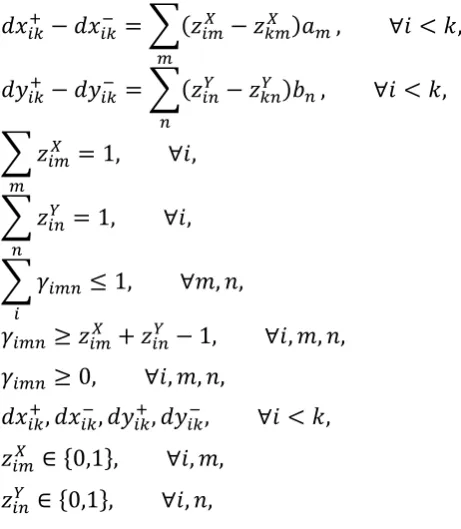
where denotes horizontal coordinate of center of column and denotes vertical coordinate of center of row with respect to the origin. Objective function (8) minimizes the total material handling cost. Constraints (9) and (10) linearize the absolute value term in the horizontal and vertical distance function, constraints (11) and (12) ensure that each facility is assigned to only one column and row, respectively. Constraint (13) restricts that each candidate point is occupied by utmost one facility. Constraints (14) linearizes the nonlinearity due to the multiplication of two binary variables (where
. ). Finally constraints (15)-(18) are the logical binary and non-negativity requirements on the decision variables.
Table 1shows the maximum number of binary and positive variables as well as maximum number of constraints, for both models. Note that in the model of QAP,| |. | |is replaced instead of | | (since
| |. | | | |).
Fig. 1. Two different approaches for assigning facilities to the candidate points
Table 1
Characteristics of the QAP, GRQAP
QAP No. Binary variables | |. | | | |. | |. | |
No. Positive variables | |. | | | |. | |. | |
No. Constraints | |. | | | | | | | |. | |. | | | | | |. | |
GRQAP No. Binary variables | | | | | |
No. Positive variables | | 2 | | 1 | |. | |
No. Constraints | | 1 | |. | | | |
| |: Number of facilities, | | | |. | |: Number of candidate points, | |: Number of columns, | |: Number of rows
1 2 3 4
5 6 7 8
9 10 11 12
3
2 M5
1
1 2 3 4
a) Numbered candidate points
3. Numerical example 1
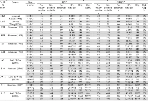
In this section, several small and small-to-medium scale problems have been selected from the literature in order to compare the GRQAP and QAP. In these examples it is assumed that the dimension of all facilities is1×1. All problem instances were solved by using CPLEX 10 on a PC with 2.4 GHz CPU, 2 GB memory, and Windows 7 operating system. The computational results have been reported in Table 2.
Table 2
Computational results of small and small-to-medium scale problems to compare QAP and GRQAP
Proble m name
Source Size QAP GRQAP
i×m×n No.
binary variable s No. positive variable s No. constraint s CPU time (s)
Obj. Opt. Gap% No. binary variable s No. positive variable s No. constraint s CPU time (s)
Obj. Opt. Gap
%
HK4 Heragu & Kusiak(1991)
4×4×1 16 16 24 0.180 40 0% 20 40 40 0.055 40 0%
4×2×2 16 16 24 0.096 34 0% 16 40 40 0.060 34 0%
LW5 Love &
Wong(1976)
5×5×1 25 25 35 0.174 30 0% 30 65 60 0.059 30 0%
5×3×2 30 30 41 0.181 28 0% 25 70 66 0.168 28 0%
S8H Simmons(1969) 8×8×1 64 64 80 3.367 200 0% 72 176 144 1.014 200 0%
8×4×2 64 64 80 5.523 143 0% 48 176 144 3.096 143 0%
8×3×3 72 72 89 18.384 138 0% 48 184 153 11.965 138 0%
S8H Simmons(1969) 8×8×1 64 64 80 11.561 488 0% 72 176 144 5.531 488 0%
8×4×2 64 64 80 15.183 325 0% 48 176 144 7.835 325 0%
8×3×3 72 72 89 38.504 313 0% 48 184 153 21.877 313 0%
S9 Simmons(1969) 9×9×1 81 81 99 108.180 734 0% 90 225 180 29.485 734 0%
9×5×2 90 90 109 404.782 490 0% 63 234 190 224.252 490 0%
9×3×3 81 81 99 138.551 441 0% 54 225 180 80.783 441 0%
S9H Simmons(1969) 9×9×1 81 81 99 84.852 423 0% 90 225 180 8.141 423 0%
9×5×2 90 90 109 194.995 294 0% 63 234 190 69.594 294 0%
9×3×3 81 81 99 90.176 274 0% 54 225 180 38.335 274 0%
A9 Adel El-Baz
(2004)
9×9×1 81 81 99 6.018 65239 0% 90 225 180 1.634 65239 0%
9×5×2 90 90 109 9.874 4854 0% 63 234 190 9.959 4854 0%
9×3×3 81 81 99 11.064 4818 0% 54 225 180 9.783 4818 0%
S10 Simmons (1969) 10×10×1 100 100 120 373.243 492 0% 110 280 220 16.644 492 0%
10×5×2 100 100 120 585.348 334 0% 70 280 220 193.374 334 0%
10×4×3 120 120 142 1614.011 315 0% 70 300 242 970.784 315 0%
LW11 Love & Wong
(1976) 11×11×1 11×6×2 132 121 121 132 143 155 2744.664063.60 1207795 26.36%0% 132 88 341 352 264 276 3631.2774.876 1207793 0% 0%
11×4×3 132 132 155 4662.41 725 0% 77 352 276 5256.94 725 0%
S11 Simmons (1969) 11×11×1 121 121 143 3509.11 1207 29.68% 132 341 264 105.261 1207 0%
11×6×2 132 132 155 2889.62 793 26.84% 88 352 276 1485.52 793 0%
11×4×3 132 132 155 2922.51 725 29.27% 77 352 276 7220.92 725 0%
A12 Adel El-Baz
(2004)
12×12×1 144 144 168 1893.83 11055 0% 156 408 312 40.661 11055 0%
12×6×2 144 144 168 1877.24 8460 41.98% 96 408 312 517.237 8460 0%
12×4×3 144 144 168 3308.07 8040 15.66% 84 408 312 1239.52 8040 0%
i: number of facilities, m: number of rows, n: number of columns * in this case solver was interrupted due to insufficient physical memory
All numerical instances were solved optimally by the GRQAP; while the QAP could not solve some cases optimally and the solver was interrupted due to insufficient physical memory. It means that the GRQAP needs relatively less physical memory. In addition, the results show that the GRQAP can solve the problem in shorter computational time than QAP. The average improvement percent in solution time(except the cases which weren’t solved optimally) is 52.52%.So it is concluded that the GRQAP can solve small and small-to-medium scale problems about two times as fast as the QAP.
4. Formulating the integrated facility layout problem
In this section, the integrated facility layout problem (IFLP) is formulated, under the following notations:
Indices:
, Index of departments
Index of columns Index of rows
Model parameters:
number of departments width of department height of department
number of facilities of department number of rows of department number of columns of department
length of center of column of cell in x-axis with respect to the left edge of cell length of center of row of cell in y-axis with respect to the down edge of cell least horizontal distance between department and department
least vertical distance between department and department
amount of material flow between facility of department and facility of department material handling cost per unit flow per unit distance traveled between facility of department and facility of department
a large number
Decision variables:
, coordinates of center of department
1 if department is located vertically, 0 otherwise
1 if facility is assigned to column of department , 0 otherwise 1 if facility is assigned to row of department , 0 otherwise
horizontal distance between facility of department and facility of department vertical distance between facility of department and facility of department
The mathematical model:
As it was concluded in the previous section, in contrast with the traditional QAP, the GRQAP can solve problems in a shorter computational time and with less physical memory. After combining GRQAP and continuous layout model and applying some standard linearization methods, the IFLP is formulated as the following MIP model:
IFLP:
.
.
, 1, … , , 1, … , 1, 1, … ,
(20)
, 1, … , , 1, … , 1, 1, … ,
(21)
1
2 1 2 2 2 . . ,
1, … , 1, 1, … , , 1, … , , 1, … , (22)
2 2 1 2 1 2 . . ,
1, … , 1, 1, … , , 1, … , , 1, … , (23)
. . 1 . . 1 , 1, … , ,
1, … , (24)
. . , 1, … , , 1, … , (25)
1 , 1, … , , 1, … ,
(26)
1 , 1, … , , 1, … ,
(27)
1 , 1, … , , 1, … , , 1, … ,
(28)
1, 1, … , , 1, … , , 1, … , , 1, … , (29)
. . 1
2 1 . 1 . , 1, … , 1,
1, … , (30)
1 . 1
2 1 . 1 . , 1, … , 1,
1, … , (31)
. 1 1
2 . 1 . 1 , 1, … , 1,
1, … , (32)
1 1 1
2 . 1 . 1 ,
1, … , 1, 1, … , (33)
, , , 0, 1, … , , 1, … , , 1, … , , 1, … , (34)
, 1, … , , 1, … , (35)
, 0,1 , 1, … , 1, 1, … , (36)
, 0, 1, … , (37)
0,1 , 1, … , (38)
0,1 , 1, … , , 1, … , , 1, … , (39)
0,1 , 1, … , , 1, … , , 1, … , (40)
The objective function (19) minimizes the total material handling cost, including inter and intra-department material handling costs. Note that in the intra-intra-department material handling cost function,
the indexes of have been reduced to , (e.g. or ). Constraints (20) and
(21) linearize the absolute value term in the intra-department rectilinear distance function, constraints (22) and (23) linearize the absolute value term in the inter-department rectilinear distance function, constraints (24) and (25) linearize the quadratic term due to the product of a binary variable and a free expression within the absolute value terms in constraints (22) and (23) i.e. ∑ .
∑ . , where is a free auxiliary variable. This quadratic term has been linearized by applying the following proposition.
Proposition 1. Set of constraints (24) and (25) linearize the following quadratic
term: ∑ . ∑ . .
Proof. This can be shown for each of two possible cases:
Case 1: 1. In this case constraints (24) and (25) are reduced to the following constraints:
. . . . , 1, … , , 1, … ,
, 1, … , , 1, … ,
Therefore it is concluded that is equal to ∑ . ∑ . .
Case 2: 0. In this case constraints (24) and (25) are reduced to the following constraints:
, 1, … , , 1, … ,
0 0, 1, … , , 1, … ,
Thus it is concluded that 0. □
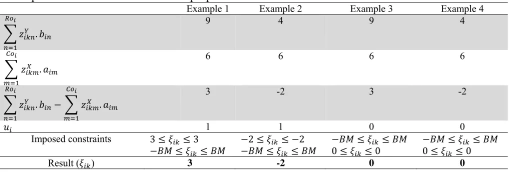
Also, Table 3 illustrates how the linearization in Proposition 1 works through four numerical examples.
Table 3
Examples to the linearization stated in proposition 1
Example 1 Example 2 Example 3 Example 4
.
9 4 9 4
.
6 6 6 6
. .
3 -2 3 -2
1 1 0 0
Imposed constraints 3 3 2 2
0 0 0 0
Result ( ) 3 -2 0 0
candidate point in each department can be occupied by utmost one facility, constraint (29) linearizes the nonlinearity of . , where the auxiliary variable is equal to . . Set of constraints (30)-(33) ensure that departments do not overlap, also in these constraints, , and are auxiliary binary variables. Finally, constraints (34)-(41) are the logical binary and non-negativity requirements on the decision variables.
5. Numerical example 2
As it was mentioned before, one of the applications of the proposed model is in the layout design of CMS i.e. after specifying machine cells and part families. To show this application, several small, medium and large scale numerical examples have been selected from the literature of CMS, and the IFLP is applied on them. Note that in these examples expression of ‘cell’ is equivalent to‘department’
and term of ‘machine’ is equivalent to ‘facility’.
5.1. Small scale problems
The first small scale problem (S1) has been selected from Akturk & Turkcan (2000); they concluded that 3 machine cells must be formed to produce 20 parts. The information corresponds to machine cells and material flow cost ( . ) among machines has been given in Table 4. It is necessary to mention that this table has been obtained according to demand of parts, processing routes of parts and inter and intra-cell material handling cost, that are exist in the reference paper.
Table 4
The material flowcost among machines (problem S1)
1-1 1-2 1-3 1-4 1-5 1-6 2-1 2-2 2-3 3-1 3-2 3-3 3-4
1-1 0.0 1104.8 0 0 0 391.3 0 0 0 0 0 0 0
1-2 0 1952.1 1192.9 0 924.8 0 0 0 0 0 0 0
1-3 0 0 0 0 0 0 0 287.6 0 0 0
1-4 0 0 0 0 0 0 0 0 0 0
1-5 0 2104.3 0 0 0 0 0 672.0 0
1-6 0 0 0 0 0 0 0 0
2-1 0 1548.8 0 0 0 368.7 0
2-2 0 2138.5 0 0 0 0
2-3 0 0 0 0 0
3-1 0 2481.1 537.6 0
3-2 0 2019.4 2229.0
3-3 0 1367.2
3-4 0
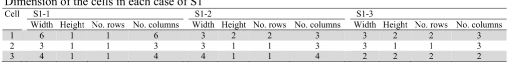
The problem S1 has been solved for different cell sizes as the following cases: S1-1, S1-2 and S1-3. Table 5 shows the dimension of each case.
Table 5
Dimension of the cells in each case of S1
Cell S1-1 S1-2 S1-3
Width Height No. rows No. columns Width Height No. rows No. columns Width Height No. rows No. columns
1 6 1 1 6 3 2 2 3 3 2 2 3
2 3 1 1 3 3 1 1 3 3 1 1 3
3 4 1 1 4 4 1 1 4 2 2 2 2
with a gap of 9%; or by comparing S1-1 and S1-2, it is concluded that the material handling cost has been reduced about 5%. Therefore, in order to attain better solution, the decision maker should consider different dimension of the cells. The next small scale problem (S2) is selected from Cheng et al. (1966); this problem contains 20 parts and 10 machines. They grouped parts into 3 part families that should be produced using 3 machine cells with 5, 3 and 4 machines in cell 1, 2 and 3 respectively. Table 6 presents the material flow among machines, for the proposed problem. In addition, the unit intra and inter-cell handling cost per unit distance is assumed 5 and 7 units, respectively. This problem has been solved in three cases, including S2-1, S2-2 and S2-3. In S2-1 the layout of machines within all cells is linear and in S2-2it is multi rows for cell 1 and 3. Also S2-3 is similar to S2-2 ,0.5 units for aisle distance.
Table 6
Material flow among machines (Problem S2)
1-1 1-2 1-3 1-4 1-5 2-1 2-2 2-3 3-1 3-2 3-3 3-4
1-1 0 148 0 0 0 310 0 0 94 0 0 32
1-2 0 246 36 122 44 0 0 0 140 0 24
1-3 0 102 122 0 0 0 0 0 0 68
1-4 0 128 0 0 24 0 0 0 36
1-5 0 0 0 82 0 0 0 142
2-1 0 130 0 18 216 0 0
2-2 0 52 0 18 0 96
2-3 0 0 0 0 662
3-1 0 96 0 0
3-2 0 234 22
3-3 0 342
3-4 0
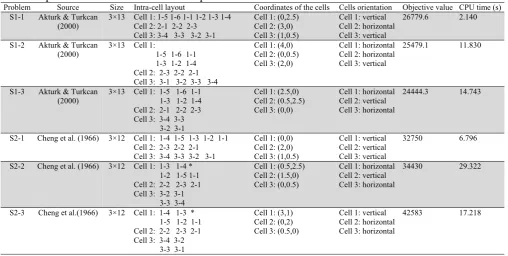
S2-1, S2-2 and S2-3 were solved optimally and the results have been summarized in Table 7. The results show that, unlike S1, by increasing the number of rows, total material handling cost has been increased.
Table 7
The computational results of small scale problems
Problem Source Size Intra-cell layout Coordinates of the cells Cells orientation Objective value CPU time (s)
S1-1 Akturk & Turkcan
(2000) 3×13 Cell 1: 1-5 1-6 1-1 1-2 1-3 1-4 Cell 2: 2-1 2-2 2-3 Cell 3: 3-4 3-3 3-2 3-1
Cell 1: (0,2.5) Cell 2: (3,0) Cell 3: (1,0.5)
Cell 1: vertical Cell 2: horizontal Cell 3: vertical
26779.6 2.140
S1-2 Akturk & Turkcan (2000)
3×13 Cell 1:
1-5 1-6 1-1 1-3 1-2 1-4 Cell 2: 2-3 2-2 2-1 Cell 3: 3-1 3-2 3-3 3-4
Cell 1: (4,0) Cell 2: (0,0.5) Cell 3: (2,0)
Cell 1: horizontal Cell 2: horizontal Cell 3: vertical
25479.1 11.830
S1-3 Akturk & Turkcan
(2000) 3×13 Cell 1: 1-5 1-6 1-1 1-3 1-2 1-4 Cell 2: 2-1 2-2 2-3 Cell 3: 3-4 3-3 3-2 3-1
Cell 1: (2.5,0) Cell 2: (0.5,2.5) Cell 3: (0,0)
Cell 1: horizontal Cell 2: vertical Cell 3: horizontal
24444.3 14.743
S2-1 Cheng et al. (1966) 3×12 Cell 1: 1-4 1-5 1-3 1-2 1-1 Cell 2: 2-3 2-2 2-1 Cell 3: 3-4 3-3 3-2 3-1
Cell 1: (0,0) Cell 2: (2,0) Cell 3: (1,0.5)
Cell 1: vertical Cell 2: vertical Cell 3: vertical
32750 6.796
S2-2 Cheng et al. (1966) 3×12 Cell 1: 1-3 1-4 * 1-2 1-5 1-1 Cell 2: 2-2 2-3 2-1 Cell 3: 3-2 3-1 3-3 3-4
Cell 1: (0.5,2.5) Cell 2: (1.5,0) Cell 3: (0,0.5)
Cell 1: horizontal Cell 2: vertical Cell 3: horizontal
34430 29.322
S2-3 Cheng et al.(1966) 3×12 Cell 1: 1-4 1-3 * 1-5 1-2 1-1 Cell 2: 2-2 2-3 2-1 Cell 3: 3-4 3-2 3-3 3-1
Cell 1: (3,1) Cell 2: (0,2) Cell 3: (0.5,0)
Cell 1: vertical Cell 2: horizontal Cell 3: horizontal
42583 17.218
5.2. Medium scale problems
In this section in order to evaluate the performance of IFLP on medium scale problems, several numerical examples are selected from Adil & Rajamani (2000), Harhalakis et al.(1990) and Ramabhatta & Nagi (1996).
The first medium scale problem has been selected from Adil and Rajamani (2000). They implemented a simulated annealing algorithm (SAA) on a CMS problem from Harhalakis et al. (1990) with 20 parts and 20 machines, to minimize the number of inter-cell moves. They concluded that the solution obtained by the SAA is better than the solution reported by Harhalakis et al. (1990). They specified 3 machine cells with 13 inter-cell moves, while Harhalakis et al. (1990) specified 4 machine cells with 14 inter-cell moves. Table 8 and Table 9 show the material flow among machines based on the solutions reported by Adil & Rajamani (2000) and Harhalakis et al. (1990), respectively. In these problems the material flow are calculated according to processing routes of parts. In addition, it is assumed that the unit inter and intra-cell material handling cost per unit distance are 15 and 10 units, respectively.
Table 8
Material flow among machines (Problem M1)
1-1 1-2 1-3 1-4 1-5 1-6 2-1 2-2 2-3 2-4 2-5 2-6 2-7 3-1 3-2 3-3 3-4 3-5 3-6 3-7 1-1 0 5 0 0 0 0 0 0 0 0 0 0 1 0 0 0 0 0 0 0
1-2 0 2 0 2 0 0 1 1 0 0 0 0 0 0 0 0 0 0 0
1-3 0 3 0 1 0 0 1 0 0 0 0 0 0 0 1 0 0 0
1-4 0 1 0 0 0 0 0 0 0 1 1 0 0 0 0 0 0
1-5 0 0 0 1 0 0 0 0 0 1 0 0 0 0 1 0
1-6 0 0 0 0 0 0 0 0 0 0 0 0 1 0 0
2-1 0 2 2 1 0 0 0 0 0 0 0 0 0 0
2-2 0 2 0 0 0 0 0 0 0 0 0 0 0
2-3 0 2 0 0 1 0 0 0 0 0 0 0
2-4 0 2 0 0 0 0 0 0 0 0 1
2-5 0 3 1 0 0 0 0 0 0 0
2-6 0 1 0 0 0 0 1 0 0
2-7 0 0 0 0 0 0 0 0
3-1 0 3 0 0 0 2 0
3-2 0 1 0 0 1 0
3-3 0 3 1 0 0
3-4 0 2 0 1
3-5 0 0 1
3-6 0 0
3-7 0
Table 9
Material flow among machines (Problem M2)
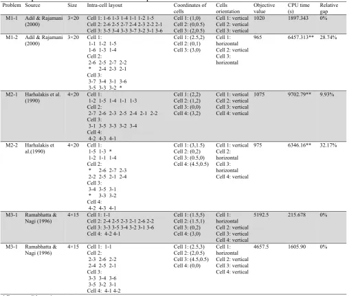
Each of solutions reported by Adil & Rajamani(2000) and Harhalakis et al. (1990) are studied under two cases. In M1-1 and M2-1, the layout of machines within all cells is single row (linear), and in M1-2 and M2-2 it is multi rows. The solutions of these cases have been summarized in Table 10.The problems were solved with good optimality gap and the results show that M1-2 gives the smallest material handling cost.
The next medium scale problem, M3 has been selected from Ramabhatta and Nagi (1996), they specified 4 machine cells with 1, 6, 6 and 2 machines in the cells 1-4 respectively. They developed a CMS model to minimize the number of inter-cell material flow instead of the inter-cell material handling cost, and finally it was realized that the total number of inter-cell movements is 83. Now this problem is solved by the IFLP (considering inter and intra-cell material handling cost). It is assumed that the unit inter and intra-cell handling cost per unit distance are 7 and 5 units, respectively, also width of the aisle distance is assumed 0.5 units. M3 is studied under two cases, linear intra-cell layout (M3-1) and multi row intra-cell layout (M3-2). Table 10 shows the optimum solutions for M3-1 and M3-2. Both cases were solved optimally and finally it was concluded that in this problem multi row layout is better than linear layout with a gap of 10%.
Table 10
The computational results of medium scale problems
Problem Source Size Intra-cell layout Coordinates of
cells Cells orientation Objective value CPU time (s) Relative gap M1-1 Adil & Rajamani
(2000)
3×20 Cell 1: 1-6 1-3 1-4 1-1 1-2 1-5 Cell 2: 2-6 2-5 2-7 2-4 2-3 2-2 2-1 Cell 3: 3-5 3-4 3-3 3-7 3-2 3-1 3-6
Cell 1: (1,0) Cell 2: (0,0.5) Cell 3: (2,0.5)
Cell 1: vertical Cell 2: vertical Cell 3: vertical
1020 1897.343 0%
M1-2 Adil & Rajamani (2000)
3×20 Cell 1: 1-1 1-2 1-5 1-6 1-3 1-4 Cell 2:
2-6 2-5 2-7 2-2 * 2-4 2-3 2-1 Cell 3:
3-7 3-4 3-1 3-6 3-5 3-3 3-2 *
Cell 1: (2.5,2) Cell 2: (0,1) Cell 3: (3,0)
Cell 1: horizontal Cell 2: vertical Cell 3: horizontal
965 6457.313** 28.74%
M2-1 Harhalakis et al. (1990)
4×20 Cell 1:
1-2 1-5 1-4 1-1 1-3 Cell 2:
2-7 2-6 2-3 2-5 2-4 2-1 2-2 Cell 3:
3-1 3-5 3-3 3-2 3-4 Cell 4:
4-2 4-3 4-1
Cell 1: (2,2) Cell 2: (1,2) Cell 3: (0,0) Cell 4: (3,2)
Cell 1: vertical Cell 2: vertical Cell 3: vertical Cell 4: vertical
1075 9702.79** 9.93%
M2-2 Harhalakis et al.(1990)
4×20 Cell 1: 1-5 1-3 * 1-2 1-1 1-4 Cell 2:
* 2-6 2-7 2-3 2-2 2-5 2-1 2-4 Cell 3:
3-4 3-5 3-1 * 3-3 3-2 Cell 4:
4-2 4-3 4-1
Cell 1: (3,1.5) Cell 2: (0,2) Cell 3: (0.5,0) Cell 4: (4.5,0.5)
Cell 1: vertical Cell 2: horizontal Cell 3: horizontal Cell 4: vertical
975 6346.16** 32.17%
M3-1 Ramabhatta & Nagi (1996)
4×15 Cell 1: 1-1
Cell 2: 2-4 2-5 2-3 2-1 2-6 2-2 Cell 3: 3-3 3-5 3-4 3-2 3-1 3-6 Cell 4: 4-2 4-1
Cell 1: (1.5,5) Cell 2: (1.5,1) Cell 3: (0,2) Cell 4: (3,0)
Cell 1: horizontal Cell 2: vertical Cell 3: vertical Cell 4: vertical
5192.5 215.678 0%
M3-1 Ramabhatta &
Nagi (1996) 4×15 Cell 1: 1-1 Cell 2: 2-3 2-6 2-2 2-4 2-5 2-1 Cell 3:
3-3 3-4 3-6 3-5 3-2 3-1 Cell 4: 4-1 4-2
Cell 1: (2.5,3) Cell 2: (2,0.5) Cell 3: (4.5,0.5) Cell 4: (0,0)
Cell 1: horizontal Cell 2: vertical Cell 3: vertical Cell 4: vertical
4657.5 1605.90 0%
* Empty candidate point
5.3. Large scale problems
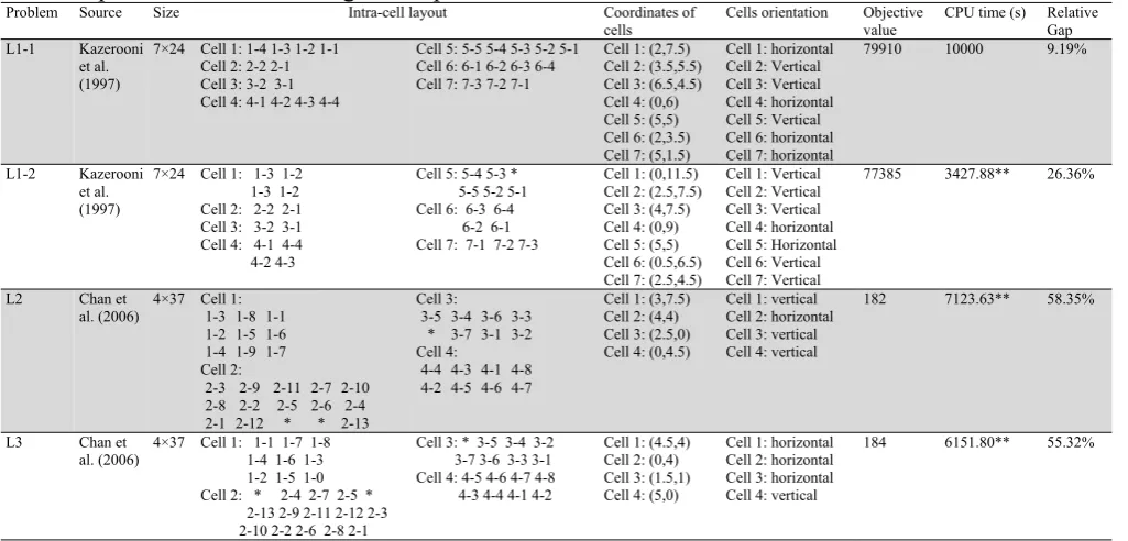
The first large scale problem has been selected from Kazerooni et al. (1997), they specified 7 machine cells with 4, 2, 2, 4, 5, 4 and 3 machines in the cells 1-7, respectively. To see the data sets, including processing routes and demand of parts, in order to specify material flow among machines, refer to Kazerooni et al. (1997). The unit intra and inter-cell material handling cost per unit distance are assumed 5 and 10 units, respectively; also the aisle distance is assumed 0.5 units. This problem has been solved in two conditions, in the first condition i.e. L1-1, the layout of machines within all cells is single row and in the next one i.e. L1-2 the layout of machines in cells 1, 4, 5 and 6 are multi rows and in the remaining cells are single row. The optimum layout of L1-1 and L1-2 has been presented in Table 12. L1-1 was interrupted after 10000 seconds, while L1-2 was terminated by the solver due to insufficient physical memory after 3927 seconds. Amount of material handling cost for L1-1 (i.e. single row layout) is 79910 with an optimality gap of 9.19%; while for L1-2 it is 77385 with an optimality gap of 28.98%. Therefore, it is concluded that for the problem presented by Kazerooni et al. (1997), the multi rows layout is better than single row layout. The next large scale problems (L2 and L3) have been selected from Chan et al. (2006).They studied a two stage CMS problem on an industrial case with 37 machines and 30 parts, where the machine cells and part families are formed in the first stage, and cell sequencing is established in the second stage. They founded two different solutions for their problem (see Table 11) and investigated different cells sequence in order to find the best sequence of the cells how total intercellular part movement being minimized. Finally, they realized that the optimal objective value for the both solutions is equal to 21.
Table 11
Presented machine cells by Chan et al. (2006) as well as machine indexes used in this paper Problem Cell number Machines (Source paper) Machines (This paper)
L2 1 3, 4, 15, 19, 24, 34, 35, 36, 37 1-1, 1-2, 1-3, 1-4, 1-5, 1-6, 1-7, 1-8, 1-9
2 7, 8, 9, 10, 11, 12, 13, 16, 18, 20, 21, 26, 31 2-1, 2-2, 2-3, 2-4, 2-5, 2-6, 2-7, 2-8, 2-9, 2-10, 2-11, 2-12, 2-13 3 14, 17, 22, 27, 28, 29, 30 3-1, 3-2, 3-3, 3-4, 3-5, 3-6, 3-7
4 1, 2, 5, 6, 23, 25, 32, 33 4-1, 4-2, 4-3, 4-4, 4-5, 4-6, 4-7, 4-8 L3 1 1, 5, 14, 17, 22, 29, 30 1-1, 1-2, 1-3, 1-4, 1-5, 1-6, 1-7
2 3, 4, 15, 19, 24, 34, 35, 36, 37 2-1, 2-2, 2-3, 2-4, 2-5, 2-6, 2-7, 2-8, 2-9 3 2, 6, 23, 25, 27, 28, 32, 33 3-1, 3-2, 3-3, 3-4, 3-5, 3-6, 3-7, 3-8
4 7, 8, 9, 10, 11, 12, 13, 16, 18, 20, 21, 26, 31 4-1, 4-2, 4-3, 4-4, 4-5, 4-6, 4-7, 4-8, 4-9, 4-10, 4-11, 4-12, 4-13
Table 12
The computational results of large scale problems
Problem Source Size Intra-cell layout Coordinates of
cells Cells orientation Objective value CPU time (s) Relative Gap L1-1 Kazerooni
et al. (1997)
7×24 Cell 1: 1-4 1-3 1-2 1-1 Cell 2: 2-2 2-1 Cell 3: 3-2 3-1 Cell 4: 4-1 4-2 4-3 4-4
Cell 5: 5-5 5-4 5-3 5-2 5-1 Cell 6: 6-1 6-2 6-3 6-4 Cell 7: 7-3 7-2 7-1
Cell 1: (2,7.5) Cell 2: (3.5,5.5) Cell 3: (6.5,4.5) Cell 4: (0,6) Cell 5: (5,5) Cell 6: (2,3.5) Cell 7: (5,1.5)
Cell 1: horizontal Cell 2: Vertical Cell 3: Vertical Cell 4: horizontal Cell 5: Vertical Cell 6: horizontal Cell 7: horizontal
79910 10000 9.19%
L1-2 Kazerooni et al. (1997)
7×24 Cell 1: 1-3 1-2 1-3 1-2 Cell 2: 2-2 2-1 Cell 3: 3-2 3-1 Cell 4: 4-1 4-4 4-2 4-3
Cell 5: 5-4 5-3 * 5-5 5-2 5-1 Cell 6: 6-3 6-4 6-2 6-1 Cell 7: 7-1 7-2 7-3
Cell 1: (0,11.5) Cell 2: (2.5,7.5) Cell 3: (4,7.5) Cell 4: (0,9) Cell 5: (5,5) Cell 6: (0.5,6.5) Cell 7: (2.5,4.5)
Cell 1: Vertical Cell 2: Vertical Cell 3: Vertical Cell 4: horizontal Cell 5: Horizontal Cell 6: Vertical Cell 7: Vertical
77385 3427.88** 26.36%
L2 Chan et
al. (2006) 4×37 Cell 1: 1-3 1-8 1-1 1-2 1-5 1-6 1-4 1-9 1-7 Cell 2:
2-3 2-9 2-11 2-7 2-10 2-8 2-2 2-5 2-6 2-4 2-1 2-12 * * 2-13
Cell 3: 3-5 3-4 3-6 3-3
* 3-7 3-1 3-2 Cell 4:
4-4 4-3 4-1 4-8 4-2 4-5 4-6 4-7
Cell 1: (3,7.5) Cell 2: (4,4) Cell 3: (2.5,0) Cell 4: (0,4.5)
Cell 1: vertical Cell 2: horizontal Cell 3: vertical Cell 4: vertical
182 7123.63** 58.35%
L3 Chan et
al. (2006) 4×37 Cell 1: 1-1 1-7 1-8 1-4 1-6 1-3 1-2 1-5 1-0 Cell 2: * 2-4 2-7 2-5 * 2-13 2-9 2-11 2-12 2-3 2-10 2-2 2-6 2-8 2-1
Cell 3: * 3-5 3-4 3-2 3-7 3-6 3-3 3-1 Cell 4: 4-5 4-6 4-7 4-8 4-3 4-4 4-1 4-2
Cell 1: (4.5,4) Cell 2: (0,4) Cell 3: (1.5,1) Cell 4: (5,0)
Cell 1: horizontal Cell 2: horizontal Cell 3: horizontal Cell 4: vertical
184 6151.80** 55.32%
Now the IFLP is imployed to solve the proposed problem by Chan et al. (2006). It is assumed that the unit inter and intra-cell material handling cost per unit distance is 2 and 1 units, respectively, also the aisle distance is assumed 0.5 units.
L2 and L3 were solved and the results have been illustrated in Table 12. Unfortunately, these problems have not been solved with good optimality gap and the relative gaps are 58.35% and 55.32% for L2 and L3, respectively. However, the primary results almost support the equality of L2 and L3, which was reported by Chan et al. (2006).
6. A heuristic method for large scale problems
In order to solve large scale problems in a short amount of time, a heuristic method have been developed. In this heuristic method, the integrated model is decomposed into three sub models. The first submodel (Model F1) creates a primary department layout, the second one (Model F2) uses the outputs of Model F1 to assign facilities to the existent department layout, then the third model (Model F3) uses the outputs of Model F2 to re-design the department layout and improve the inter-department material handling costs. Again, model F2 is implemented to re-assign facilities to the existence layout, in order to minimize total material handling costs. This procedure between Model F2 and Model F3 continues, until no further improvement resulted in the objective function. The stages of proposed heuristic are explained in detail in the next stages.
6.1. Stage 1
In this stage, a primary department layout is created according to the following MIP model.
Model F1:
Min
(42)
subject to:(30)-(33) and (36)-(38)
, , (43)
, , (44)
, , , 0, , (45)
In the above model, is total material flow cost between department and department , and is
calculated as follows: ∑ ∑ . ; also and measure the
horizontal and vertical distances between department and department , respectively, all remaining parameters are the same before defined. After solving Model F1, total material handling cost is set to
∞ and the solutions i.e. , and are placed as the inputs of the next model (Model F2).
6.2. Stage 2
In this stage, facilities are arranged within the existent department layout according to the following MIP model.
Model F2:
subject to:(20)-(23), (26)-(29), (34) and (39)-(41)
2 1 . .
1 . . , 1, … , ,
1, … , , 1, … , , 1, … , (46)
2 . 1 .
. 1 . , 1, … , ,
1, … , , 1, … , , 1, … , (47)
where , and represent existent department layout (obtained by Model F1 or the next model i.e. Model F3). After solving Model F2, if the resulted objective value i.e. becomes better than current objective value i.e. then and the main outputs of Model F2 i.e. ̃ , ̃ , are placed as the inputs of Model F3, otherwise the procedure is terminated.
6.3. Stage 3
In this stage the department layout are re-designed according to Model F3; in fact this model changes the position and orientation of departments in order to improve the inter-department material handling cost. In this submodel there are eight states for each department with respect to other departments that must be considered in the mathematical model, these states have been illustrated in Fig. 2.
Fig. 2. Eight possible states for placing a department, considering layout of facilities within the department
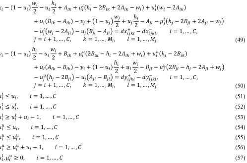
After applying standard linearization methods Model F3 is formulated as the following MIP model:
Model F3:
min .
(48)
M4 M5 M5 M4 M1 M2 M3 M3 M2 M1
M1 M2 M3 M3 M2 M1 M4 M5 M5 M4
M3 M1 M4 M3 M4 M1
M2 M5 M2 M5 M5 M2 M5 M2
subject to: (30-(34) and (36)-(38)
1
2 2 2 2 2
1
2 2 2 2
2 , 1, … , ,
1, … , , 1, … , , 1, … , (49)
1
2 2 2 2 2
1
2 2 2 2
2 , 1, … , ,
1, … , , 1, … , , 1, … , (50)
, 1, … , (51)
, 1, … , (52)
1, 1, … , (53)
, 1, … , (54)
, 1, … , (55)
1, 1, … , (56)
, 0, 1, … , (57)
Note that, since in Model F3 the layout of facilities within the departments is fixed therefore the intra-department material handling cost is constant and it is calculated as follows:
∑ ∑ ∑ | | | | , where ∑ ̃ . ,
∑ ̃ . .Also in the above model , and are related to the direction of department . Table 13 illustrates the eight possible states resulted by these variables for a hypothetical facility within a department. After solving Model 3, if the resulted objective value i.e. be better than current objective value i.e. then and the main outputs of Model 3 i.e. ̃ , ̃ , are placed as the inputs of Model F2, otherwise the procedure is terminated. Fig. 3. illustrates the flowchart of proposed heuristic method.
Table 13
The coordinates of a hypothetical facility within a department with respect to the direction of the department
States width height
1 0 0 0
2 2
2 0 0 1
2 2
3 0 1 0
2 2
4 0 1 1
2 2
5 1 0 0
2 2
6 1 0 1
2 2
7 1 1 0
2 2
8 1 1 1
Fig. 3. Flowchart of proposed heuristic method
7. Numerical example.3
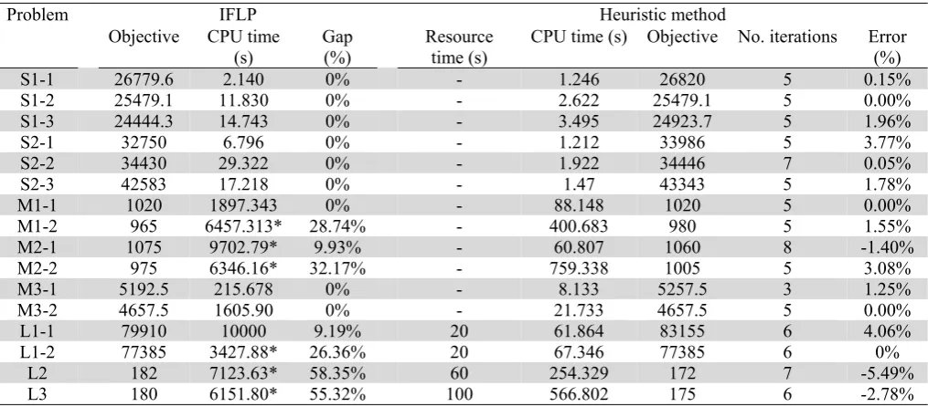
In this section, the proposed heuristic method is implemented to solve the same problems presented in section 5. The results are compared against the IFLP. The computational results have been summarized in Table 14.The column of resource time shows the maximum time for each iteration of the heuristic
method. Also the error percent column ‘Error (%)’has been calculated as follows:
100.
Table 14
The results of the heuristic method
Problem IFLP Heuristic method
Objective CPU time
(s) Gap (%) Resource time (s) CPU time (s) Objective No. iterations Error (%)
S1-1 26779.6 2.140 0% - 1.246 26820 5 0.15%
S1-2 25479.1 11.830 0% - 2.622 25479.1 5 0.00%
S1-3 24444.3 14.743 0% - 3.495 24923.7 5 1.96%
S2-1 32750 6.796 0% - 1.212 33986 5 3.77%
S2-2 34430 29.322 0% - 1.922 34446 7 0.05%
S2-3 42583 17.218 0% - 1.47 43343 5 1.78%
M1-1 1020 1897.343 0% - 88.148 1020 5 0.00%
M1-2 965 6457.313* 28.74% - 400.683 980 5 1.55%
M2-1 1075 9702.79* 9.93% - 60.807 1060 8 -1.40%
M2-2 975 6346.16* 32.17% - 759.338 1005 5 3.08%
M3-1 5192.5 215.678 0% - 8.133 5257.5 3 1.25%
M3-2 4657.5 1605.90 0% - 21.733 4657.5 5 0.00%
L1-1 79910 10000 9.19% 20 61.864 83155 6 4.06%
L1-2 77385 3427.88* 26.36% 20 67.346 77385 6 0%
L2 182 7123.63* 58.35% 60 254.329 172 7 -5.49%
L3 180 6151.80* 55.32% 100 566.802 175 6 -2.78%
* Interrupted by the solver due to insufficient physical memory
The results show that in cases of S1-2, M1-1, M3-2 and L1-2 the objective value of the proposed heuristic is equal to that of IFLP, and in cases of M2-1, L2, L3 the heuristic method even obtained better solution than the IFLP. Also in the remaining cases, the average error percent between the IFLP
Create primary department layout using
Model F1
Assign machines to the current department layout using Model F2
Re-arrange department layout using Model F3
Let TC=∞
End
TC2<TC
TC3<TC TC=TC2
TC=TC3
No
Yes
and heuristic method is about 2.2%. Therefore, it is deduced that the proposed heuristic is an efficient method for solving problems in reasonable time.
7. Conclusions
In this paper, an integrated layout model was developed to incorporate inter and intra-department layout. First, a modified version of QAP, namely GRQAP, with fewer binary variables was developed; in contrast to traditional QAP, the GRQAP can solve the problems in a shorter computational time and with less physical memory. Then the IFLP was formulated based on the GRQAP in order to minimize total material handling cost. Several numerical examples were selected from the literature of CMS and the IFLP applied on them. Also due to the complexity of integrated model, an efficient heuristic method was developed in order to solve large scale problems in short amount of time. Finally, it was deduced that in contrast with the ICFLP, the proposed heuristic could even obtain better solution over a short amount of time.
References
Adel El-Baz, M. (2004). A genetic algorithm for facility layout problems of different manufacturing environments. Computers & Industrial Engineering, 47, 233–246.
Adil, G. K., & Rajamani, D. (2000). The Trade-Off Between intracell and intercell moves in group technology cell formation. Journal of Manufacturing Systems, 19 (5), 305-317.
Akturk, M. S., & Turkcan, A. (2000). Cellular manufacturing system design using a holonistic approach. International Journal of Production Research, 38 (10), 2327-2347.
Chan, F. T., Lau, K., Chan, P., & Choy, K. (2006). Two-stage approach for machine-part grouping and cell layout problems. Robotics and Computer-Integrated Manufacturing, 22, 217–238.
Cheng, C. H., Madan, M. S., & Motwani, J. (1966). Knapsack-based algorithm for designing cellular manufacturing systems. The Journal of Operation Research Society, 47 (12), 1648-1476.
Chiang, C.-P., & Lee, S.-D. (2004). Joint determination of machine cells and linear intercell layout.
Computers & Operations Research, 31, 1603–1619.
Commander, C. W. (2003). A Survey of the Quadratic Assignment Problem, with Applications. The University of Florida.
Drira, A., Pierreval, H., & Hajri-Gabouj, S. (2007). Facility layout problems: A survey. Annual
Reviews in Control, 31, 255–267.
Harhalakis, G., Nagi, R., & Proth, J. M. (1990). An Eflicient Heuristic in Manufacturing Cell Formation for Group Technology Applications. International Journal of Prduction Research, 28 (1), 185-198.
Heragu, S. S., & Kusiak, A. (1991). Effcient models for the facility layout problem. European Journal
of Operational Research, 53, 1-13.
Heragu, S. S., & Kusiak, A. (1988). Machine layout problem in flexible manufacturing systems.
Operations Research, 36 (2), 258–268.
Hicks, C. (2006). A Genetic Algorithm tool for optimising cellular or functional layouts in the capital goods industry. International Journal of Production Economics, 104, 598–614.
Kaku, B., Thompson, G., & Baybars, I. (1988). A heuristic method for the multi-story layout problem.
European Journal of Operational Research, 37, 384–397.
Kaufmann, L., & Broeckx, F. (1978). An algorithm for the quadratic assignment problem using Benders’ decomposition. European Journal of Operational Research, 2, 204–211.
Kazerooni, M. L., Luong, H. S., & Abhary, K. (1997). A genetic algorithm based cell design considering alternative routing. International Journal of Computational Integrated Manufacturing
Systems, 10 (2), 93–107.
Kochhar, J. S., Foster, B. T., & Heragu, S. S. (1998). A GENETIC ALGORITHM FOR THE
UNEQUAL AREA FACILITY LAYOUT PROBLEM. Computers & Operations Research, 25
Konak, A., Kulturel-Konak, S., Norman, B. A., & Smith, A. E. (2006). Anewmixed integer programming formulation for facility layout design using flexible bays. Operations Research
Letters, 34, 660 – 672.
Koopmans, T. C., & Beckmann, M. J. (1957). Assignment problems and the location of economic activities. Econometrica, 25, 53–76.
Kusiak, A., & Heragu, S. (1987). The facility layout problem. European Journal of Operational
Research, 29, 229–251.
Love, R., & Wong, J. (1976). On solving a one-dimensional allocation problem with integer programming. Information Processing and Operations Research, 14 (2), 139–143.
Meller, R., & Gau, K. (1996). The facility layout problem: recent and emerging trends and perspectives. Journal of Manufacturing Systems, 15, 351–366.
Ramabhatta, V., & Nagi, R. (1996). An integrated formulation of manufacturing cell formation with capacity planning and multiple routings. Baltzer Journals, 1-18.
Sahni, S., & Gonzalez, T. (1976). P-complete Approximation Problems. Journal of the ACM, 23, 555-565.
Simmons, D. (1969). One-dimensional space allocation: An ordering algorithm. Operations Research, 17, 812–826.
Singh, S. P., & Sharma, R. R. (2005). A review of different approaches to the facility layout problems.
The International Journal of Advanced Manufacturing Technology, 30, 425–433.
Solimanpur, M., Vrat, P., & Shankar, R. (2005). An ant algorithm for the single row layout problem in flexible manufacturing systems.Computers & Operations Research, 3 (32), pp. 583–598.
Sule, D. R. (1994). Manufacturing facilities: location, planning, and design (2nd ed.). Boston: PWS Publishing Company.
Taghavi, A., & Murat, A. (2011). A heuristic procedure for the integrated facility layout design and flow assignment problem. Computers & Industrial Engineering, 61, 55–63.
Tavakkoli-Moghaddam, R., Javadian, N., Javadi, B., & Safaei, N. (2007). Design of a facility layout problem in cellular manufacturing systems with stochastic demands. Applied Mathematics and
Computation, 184, 721–728.
Tompkins, J. A., White, J. A., Bozer, Y. A., & Tanchoco, J. M. (2003). Facilities planning (3rd ed.).
New York: John Wiley & Sons.
Wemmerlöv, U., & Hyer, N. (1986). Procedures for the part family/machine group identification problem in cellular manufacture. Journal of Operations Management, 6, 125-147.