Patron: Her Majesty The Queen Rothamsted Research Harpenden, Herts, AL5 2JQ
Telephone: +44 (0)1582 763133 Web: http://www.rothamsted.ac.uk/
Rothamsted Research is a Company Limited by Guarantee Registered Office: as above. Registered in England No. 2393175. Registered Charity No. 802038. VAT No. 197 4201 51. Founded in 1843 by John Bennet Lawes.
Rothamsted Repository Download
A - Papers appearing in refereed journals
Parnell, S., Gottwald, T. R., Irey, M. S., Luo, W. and Van Den Bosch, F.
2011. A stochastic optimization method to estimate the spatial distribution
of a pathogen from a sample. Phytopathology. 101 (10), pp. 1184-1190.
The publisher's version can be accessed at:
•
https://dx.doi.org/10.1094/PHYTO-11-10-0311
The output can be accessed at:
https://repository.rothamsted.ac.uk/item/8qq09/a-
stochastic-optimization-method-to-estimate-the-spatial-distribution-of-a-pathogen-from-a-sample
.
© Please contact [email protected] for copyright queries.
Ecology and Epidemiology
A Stochastic Optimization Method to Estimate
the Spatial Distribution of a Pathogen from a Sample
S. Parnell, T. R. Gottwald, M. S. Irey, W. Luo, and F. van den Bosch
First and fifth authors: Centre for Mathematical and Computational Biology, Rothamsted Research, Harpenden, Herts., AL5 2JQ, UK: second author: United States Department of Agriculture, Agricultural Research Service, 2001 South Rock Road, Ft. Pierce, FL 34945: third author: U.S. Sugar Corporation, Clewiston, FL 33440: and fourth author: The Food and Environment Research Agency (FERA), Sand Hutton, York, YO411LZ, UK.
Accepted for publication 13 May 2011.
ABSTRACT
Parnell, S., Gottwald, T. R., Irey, M. S., Luo, W., and van den Bosch, F.
2011. A stochastic optimization method to estimate the spatial
distri-bution of a pathogen from a sample. Phytopathology 101:1184-1190.
Information on the spatial distribution of plant disease can be utilized to implement efficient and spatially targeted disease management inter-ventions. We present a pathogen-generic method to estimate the spatial distribution of a plant pathogen using a stochastic optimization process which is epidemiologically motivated. Based on an initial sample, the method simulates the individual spread processes of a pathogen between patches of host to generate optimized spatial distribution maps. The method was tested on data sets of Huanglongbing of citrus and was
compared with a kriging method from the field of geostatistics using the well-established kappa statistic to quantify map accuracy. Our method produced accurate maps of disease distribution with kappa values as high as 0.46 and was able to outperform the kriging method across a range of sample sizes based on the kappa statistic. As expected, map accuracy improved with sample size but there was a high amount of variation between different random sample placements (i.e., the spatial distribution of samples). This highlights the importance of sample placement on the ability to estimate the spatial distribution of a plant pathogen and we thus conclude that further research into sampling design and its effect on the ability to estimate disease distribution is necessary.
Spatially referenced information on disease incidence can be utilized to develop more efficient and effective use of disease control resources. For example, host removal radii have been implemented in recent economically significant eradication programs which work by targeting the spatial increase in asymp-tomatic infections that occur around a detected focal infection (7,17). Additionally, applications in precision agriculture have sought to minimize pesticide inputs via spatially targeted spray applications whereby applications are limited to diseased hosts and their neighbors only (19). Such methods rely on accurate information on the spatial distribution of disease. A simple but time-consuming way to determine spatial disease incidence would be to conduct an exhaustive survey of a host population. However, resource constraints usually render this unpractical and so instead it is necessary to make inferences about the spatial distribution of disease from a sample.
Although much progress has been made in nonspatial and spatially implicit methods to estimate disease incidence in plant epidemiology (13), much less work has been done on methods to generate estimated maps of disease incidence. The few plant pathological studies that have attempted to estimate the spatial distribution of disease have largely adopted techniques from geostatistics (16). These are universal methods which originate in mineral exploration and mining and use statistical models to estimate a continuous variable from a set of point samples. As such, a feature of these methods is that they are not underpinned by the epidemiological processes that shape plant disease distri-bution, such as pathogen dispersal, nor do they incorporate the spatial heterogeneity present in host populations, which are often
irregular and noncontiguous. The interaction of these two com-ponents (dispersal and host heterogeneity) can lead to complex spatial patterns that are difficult to predict (9).
In this paper an iterative stochastic optimization process is used to estimate the spatial distribution of a pathogen from a sample by explicitly simulating the individual distance-dependent spread processes between the pathogen and its host population. In doing so, the key epidemiological processes that determine the spatial distribution of a pathogen were incorporated; specifically, dis-persal and the spatial availability of the host. The method is demonstrated through a case study of Huanglongbing (HLB) in Florida (syn. citrus greening, causal agent ‘Candidatus Liberi-bacter asiaticus’), a Liberi-bacterial pathogen spread by a psyllid vector (Diaphorina citri) (4). This case study has been selected because of the current economic significance of this pathogen and also because of the availability of high quality data sets from which the performance of our method can be tested (4). The data consist of an exhaustive survey of commercial citrus plantings in Florida whereby thousands of individual trees were inspected for symp-toms of HLB disease, thus generating a complete disease map.
MATERIALS AND METHODS
In this section, we first describe the estimation method and then the data sets used to test the method. Finally, we describe the statistical approaches used to assess the performance of the method.
Estimation method. The estimation method is an iterative stochastic optimization algorithm whereby we estimate the prob-ability of disease for each unsampled individual. A host “indi-vidual” represents a single tree in the examples given in this study but could equally represent a field, patch, or any other discrete unit of host. By iterating through unsampled individuals at random, updating their probability of disease and accepting only
Corresponding author: S. Parnell; E-mail address: [email protected]
doi:10.1094 / PHYTO-11-10-0311
map-improving changes, the estimated map becomes more accu-rate with increasing iterations of the algorithm. The algorithm is as follows.
Initialization
1. The locations of all individuals in the host population are inputted and those which have been sampled are identified.
2. The disease status of sampled individuals has been deter-mined in the field/laboratory and we can allocate probabilities accordingly (i.e., either 1 if the disease is present or 0 if the disease is absent). For unsampled individuals, the probability of disease is drawn from a uniform distribution and this is used as the initial condition of the system.
3. Based on the initial condition of the system, we calculate the initial value of the objective function (i.e., the function to be minimized during iterations of the algorithm). For our purposes, the objective function is a metric describing the accuracy of the estimated map. The “estimated map” refers to the set of estimated probabilities of disease for all unsampled individuals. In practice only the disease status of sampled individuals is known and therefore this is the only information that can be used to assess the accuracy of the estimated map, i.e., to determine the objective function. For ease of explanation, the full description of the objective function is saved until after the algorithm has been outlined in full.
Iteration loop
4. Choose an unsampled individual i at random and update its probability of disease according to the function.
⎥ ⎦ ⎤ ⎢ ⎣ ⎡ μ − θ − − = ∑ ≠j
i j ij
i P d
P 1 exp exp( ) (1)
This function is a description of how the probability of disease increases with distance to, and increased disease probability of, other individuals. Here, dij is the distance between unsampled
individual i and (sampled or unsampled) individual j, where θ and µ are transmission and dispersal parameters, respectively. These parameters are unknown and are estimated in a later stage of the algorithm. Pi is the probability of disease for host individual j
during the current iteration.
5. Recalculate the objective function following the change made in step 4.
6. Determine if the new value of the objective function calcu-lated in step 5 is less than its value from the previous iteration (i.e., does it constitute an improvement in map accuracy based on the accuracy to estimate the status of sampled individuals). If it does then the change made in step 4 is accepted, otherwise the change is rejected (but see Discussion for alternative simulated annealing approach) and the previous estimated map and ob-jective function are retained.
7. Calculate if the stopping criterion is satisfied. The stopping criterion is calculated from the gradient of the objective function across previous iterations of the algorithm. If no changes can be found that significantly decrease the objective function, this gradient will approach zero. The stopping criterion is
ε < −
+m i
i OF
OF
where OFi is the value of the objective function during iteration i
of the algorithm. The number of iterations m and the value ε are selected from empirical observations of the objective function. This choice involves a trade-off between numerical accuracy and computation time. After considerable numerical experi-mentation we use m = 5,000 and ε = 0.01. If the stopping cri- terion is satisfied the algorithm is stopped and the current estimated map is the final estimated map. Otherwise steps 4 to 7 are repeated.
A remaining issue is the selection of values for the parameters θ and µ. These are chosen by repeating steps 4 to 7 over a range of
each of the parameters and selecting the combination which leads to the estimated map with the lowest objective function (i.e., the most accurate map). In this way the parameters θ and µ are esti-mated during the optimization process. The initial values and range used are found by trial and error but a simple extension to the algorithm would be to automate this process.
The objective function, calculated in steps 3 and 5 of the algorithm, is a measure of map accuracy based on how accurately we estimate the disease probability of sampled individuals. Opti-mization problems usually involve the miniOpti-mization rather than maximization of the objective function and thus for consistency we formulate the objective function such that by minimizing it we maximize map accuracy. As previously mentioned, the disease status of unsampled individuals will not be known in practice and so we have no information on how closely their estimates match their actual disease statuses. Thus, this information is not avail-able for the calculation of the objective function.
Instead, for each sampled individual, k, the probability that the individual is infected, Pk, is determined using the estimated
prob-abilities of disease from all other individuals (sampled and un-sampled), Pj.
⎥ ⎦ ⎤ ⎢ ⎣ ⎡− θ−μ − = ∑ ≠j
k j kj
k P d
P 1 exp exp( ) (2)
Note that equation 2 is approximately equivalent to equation 1, as appears in step 4 of the algorithm. However, the key difference is in the index denotations; here, dkjis the distance between sampled
individual k and all other individuals j. In contrast, equation 1 involves the calculation of dij, which is the distance between
unsampled individual i and all other individuals j. The parameters
θ and µ are the transmission and dispersal parameters as before and take the same values as in equation 1. The objective function is the deviance,which is essentially a measure of the difference between the estimate of disease at each sampled individual, Pk,
and its corresponding actual disease status, sk, ∑ = = n k k dev n deviance 1 ) ( 2 where ⎟⎟ ⎠ ⎞ ⎜⎜ ⎝ ⎛ − − − + ⎟⎟ ⎠ ⎞ ⎜⎜ ⎝ ⎛ = k k k k k k k P s s P s s dev 1 1 log ) 1 ( log
The deviance metric originates in likelihood statistics and can be used to make a comparison between binary observations and probability estimates (14). It is essentially twice the log-likeli-hood ratio of the estimated versus the actual values. The closer the estimated probability, Pk, to the actual status, sk, the smaller
the contribution to the deviance from each sampled individual k,
devk. The smaller the deviance (i.e., the objective function) the
better the overall estimated map as measured against the infor-mation we have from the sampled individuals.
We also used the geostatistical method of indicator kriging to generate maps of disease distribution from samples from the test data sets to allow a comparison of our method with more general geostatistical approaches that have been utilized in the field of plant pathology. Kriging is a form of statistical interpolation whereby unknown values are estimated from observed data. There are many different types of kriging; however, indicator kriging lends itself to the binary nature of spatial incidence data sets (i.e., where we consider a set of individuals which are either infected or not infected) (8).
ob-served. Each tree was visually assessed by a team of experienced field scouts familiar with the disease symptoms and HLB visually positive trees were confirmed by a senior scout/pathologist. For ease of reference, the HLB data sets are referred to as HLB1 (Fig. 1) and HLB2 (Fig. 2).
Assessing the accuracy of the estimated map against the true map. By simulating a random sample from the test data sets estimated maps of disease distribution can be estimated using the estimation method and then the performance of the method can be assessed by calculating how accurately the estimated probability of disease of each unsampled individual match its corresponding actual disease status. As a default we use a value of 15% as this is typical of sampling resource capabilities in the field; however, we also test the method using multiple random sample placements at a range of sample sizes from 5 to 25%. The estimated probabili-ties of disease are converted to binary presence/absence estimates using the average estimated probability threshold approach (12). That is, the average estimated probability of infection across all unsampled individuals is calculated, then it is determined if each individual is positive or negative for the disease depending on if its estimated probability is greater than or less than the average, respectively. The maps are then evaluated using the kappa statistic (2,12). The kappa statistic is a measure of the proportion of individuals correctly estimated once the probability of chance agreement has been removed (2,12) and utilizes the four elements of the confusion matrix, i.e., false-positives (fp), false-negatives (fn), true-positives (tp), and true-negatives (tn). It is calculated as follows.
C n
C tn tp
− − + = κ ( )
where n is the total number of hosts and
n
fp tn fn tn fp tp fn tp
C=( + )( + )+( + )( + )
Kappa is zero if the estimated map is equal to a randomly gen-erated map based on the mean incidence of disease in the sample (i.e., fp + fn = tp + tn), it is negative if it is worse than a randomly generated map (i.e., fp + fn > tp + tn ), positive if it is better than a randomly generated map (i.e., fp + fn < tp + tn), and unity if there is a perfect match between the estimated and true map (i.e., fp +
fn = 0).
RESULTS
In this section, we describe the results relating to the HLB test data sets. For each, we present results for one run of the esti-mation method from a randomly selected sample (Figs. 1 to 3). We then show results from further runs illustrating the effect of varying sample size and different realizations of random sample placements on the accuracy of the estimated maps and the comparison of our method with indicator kriging (Fig. 4).
Estimated maps of HLB. Two observed maps of HLB disease are presented (Figs. 1A and 2A). The maps have visually similar spatial distributions of infected trees (Figs. 1A and 2A). A random sample of 15% was taken from each (Figs. 1B and 2B) and used
Fig. 1. A, Map of the observed distribution of Huanglongbing (HLB) disease in a commercial planting in Florida as a result of exhaustive surveying (denoted as
HLB1). Infected trees are black and uninfected trees are white. B, The location of randomly selected hosts (sample size 15%) used as the input to the estimation
method. Sampled trees that were infected are black and sampled trees that were uninfected are white. C,Estimated probabilities of disease presence for all
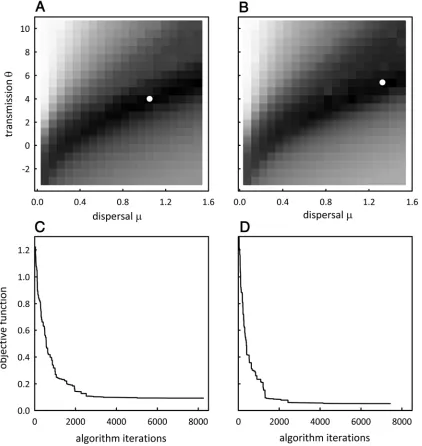
to estimate the actual maps (Figs. 1C and 2C). The estimated maps appeared visually accurate for both HLB1 (Fig. 1C) and HLB2 (Fig. 2C). The kappa-statistic analysis showed that, for the sample realizations presented, HLB1 and HLB2 were estimated with very similar accuracy with values of 0.46 and 0.44, respec-tively. The optimum values for the parameter values were differ-ent for each test data set and HLB2 had a higher dispersal, µ, and transmission value, θ (Fig. 3A and B). The number of iterations taken to reach the optimum solution was similar for both test data sets (Fig. 3C and D).
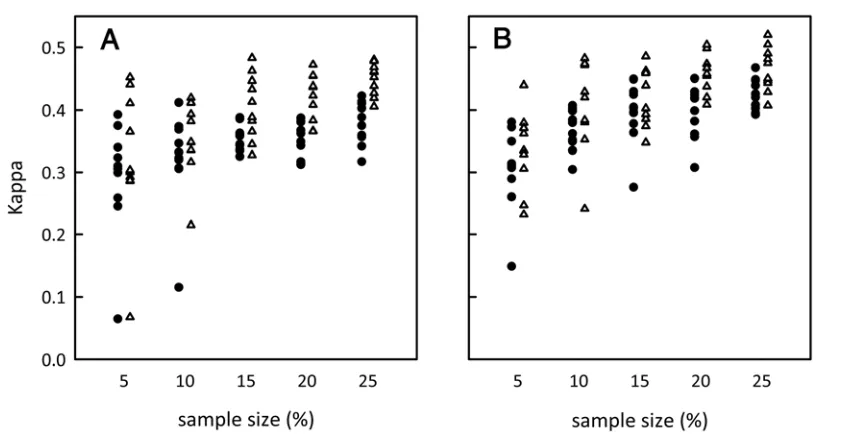
The influence of sample size and comparisons with indi-cator kriging. So far only the results for one random sample of 15% for each of the test data sets have been presented. To illu-strate the influence of varying realizations of random sample placement and sample size we estimate maps for multiple runs of the program (each using a different randomly selected sample) using different sample sizes and determine the resulting kappa statistic (Fig. 4). Here, sample placement refers to different ran-domly selected sets of sampled individuals. As expected, in gen-eral, kappa increased with increasing sample size indicating that the accuracy to estimate disease distribution improves with sample size (Fig. 4). However, we also find some variation between different sample placements. For each test data set, we show that, in at least a minority of cases, it is possible for a randomly selected sample of 5% to generate a more accurate map than a sample of 25% (Fig. 4). The estimation method outlined in this paper significantly outperformed indicator kriging for sample sizes of 20% and above and also at sample size of 10% (HLB1)
and 15% (HLB2) (Fig. 4; Table 1). When sample size was low (5%), the variation in map accuracy (kappa) was large for both our estimation method and indicator kriging and no significant difference between the two could be detected (Fig. 4; Table 1).
DISCUSSION
In this paper, we have presented a method to estimate the spatial distribution of a plant pathogen from a sample. Although the data used represent agricultural populations of citrus trees, the method retains enough generality to be applicable to many other types of pathosystems and host populations. The spatial depen-dence exhibited by epidemics means that accurate estimates of spatial pathogen distribution can facilitate the targeted deploy-ment of disease control resources. This is of key importance, not only because disease control resources are generally scarce and so must be deployed as efficiently as possible, but because patches of disease that go undetected for long periods can undergo exponential expansion and quickly become uncontrollable. Our method generates accurate estimates of pathogen spatial distribu-tion by incorporating the key determinates of spatial pathogen dynamics, that is, the dispersal characteristics of the pathogen and the distribution of the host. Moreover, in principle the method retains enough generality to be applied to any pathogen that spreads by distance-dependent processes, although this requires further testing to confirm. To our knowledge no previous study in the field of plant pathology has developed a systematic method to estimate a disease map based only on a sample. However, a small
Fig. 2. A, Map of the observed distribution of Huanglongbing (HLB) disease in a commercial planting in Florida as a result of exhaustive surveying (denoted as
HLB2). Infected trees are black and uninfected trees are white. B, The location of randomly selected hosts (sample size 15%) used as the input to the estimation
method. Sampled trees that were infected are black and sampled trees that were uninfected are white. C,Estimated probabilities of disease presence for all
number of studies have applied geostatistical techniques, such as kriging, to generate spatial estimates of disease risk based on various environmental factors including locations of known symp-tomatic plants (15). It has been demonstrated that by incorporat-ing epidemiological information on spatial pathogen dynamics it is possible to outperform general methods from the field of geostatistics (Fig. 4; Table 1). Epidemiological information has also been incorporated in recent studies using Bayesian Markov Chain Monte Carlo (MCMC) techniques to estimate dispersal and transmission parameters (3). MCMC methods are computation-ally intensive and so alternative methods have also been proposed to estimate spatial parameters (10). The focus of these studies is parameter estimation but since they also estimate the probability of infection at unobserved sites during the parameter estimation process they could be used to construct disease maps. However, we offer a simpler and more readily implementable approach that, moreover, leads directly to an estimated map of disease distribution.
The stochastic optimization process was initially achieved using a simulated annealing algorithm to avoid the problem of
local minima (11,18). During simulated annealing, changes which decrease the objective function are always retained (i.e., good changes) but additionally some changes which increase the objective function (bad changes) are also retained with a certain probability. As the algorithm progresses this probability is decre-mented with each iteration until eventually only good changes are accepted. By accepting some bad changes at the beginning of the algorithm it is possible to escape local minima (11,18). However, on examination of empirical data during the optimization process it was concluded that local minima did not present a problem in reaching the global optimum and therefore the simpler accept-reject algorithm was preferred. The objective function was determined using the deviance measure which is a function of the log-likelihood ratio of the estimated probability of disease for sampled individuals compared to their corresponding known disease status. The main reason for this is because the log-likeli-hood ratio weights against differences in the estimated value more heavily the further they are from the actual value. Although the deviance was used as a measure of accuracy during the optimi-zation process, the kappa statistic was preferred as a measure of
Fig. 3. The range of parameter values iterated over to find the combination which minimized the objective function (deviance) for A, Huanglongbing (HLB)1 and
B, HLB2. The intensity of the grayscale represents the value of the deviance and the white dots denote the location of the optimal parameter combination. C and
accuracy when comparing the estimated and actual maps for the purposes of assessing the method. The kappa statistic is a popular choice in studies of species distribution (1) and so its use here allows a comparison with such studies. Further, in practice, maps displaying probabilities of disease occurrence are less useful than maps displaying binary presence/absence data. For this reason, many studies of species distribution use threshold approaches to convert probabilities of occurrence to binary presence/absence estimates and then assess the accuracy of these estimates using a given test statistic (e.g., kappa). Additionally, since the kappa statistic was not used during the optimization procedure of our method, it allows a fair and independent comparison with the geo-statistical method of indicator kriging (Fig. 4). Here the average estimated probability approach was used to determine our threshold, which has been shown to outperform other threshold approaches such as fixed-value thresholds (12).
Our results show that it is possible to generate accurate spa-tially explicit estimates of pathogen distribution from a sample. The HLB pathogen, like many plant pathogens, are known to form clusters or aggregates as a result of a combination of long and short range dispersal events (5,6). The current method accurately maps such spatial correlations and also captures the effect of host spatial structure on disease distribution (Figs. 1 and 2). The method produced accurate disease maps with kappa values of 0.46 and 0.44 for HLB1 and HLB2, respectively, as well as outperforming the more generalized method of indicator kriging (Fig. 4). Much of the diseased pattern that was not captured is the result of random scatter from isolated, medium to long range, primary dispersal events. It should be noted that the precise location of such random events cannot be predicted by any method. That is, on average, a kappa value of zero (denoting randomness) is the maximum accuracy that can be expected in such cases. Although most pathogens disperse via spatially dependent processes, if an epidemic is characterized predomi-nantly by random scatter then spatially implicit methods to predict incidence in the population as a whole are more appropriate (13).
As expected, the accuracy to estimate pathogen distribution improves with increased sample size and also depends on the particular placement of the random sample taken (Fig. 4). How-ever, the variation between different random sample placements
(i.e., the distribution of randomly selected sampled individuals in space changes for each realization of a random sample) of the same sample size demonstrates that sample placement can have a large influence on map accuracy (Fig. 4). Some of this is un-avoidable as in practice you do not know where the disease is and occasionally and by chance a realization of a random sample will exactly capture the shape of the disease pattern. For example, we have shown that it is possible in some cases for a random sample of 5% to outperform one of 25% (Fig. 4). That is, sample place-ment can have a stronger effect than sample size. Even large random samples can lead to poorly estimated maps when popula-tion clusters or voids are, by chance, underrepresented or missed entirely. Conversely, small random samples can led to accurate maps when all population clusters are well represented by the sample, again purely by chance. A natural extension of this work is to consider how other sampling designs, e.g., regular sampling or stratified random sampling, influence the accuracy to estimate pathogen distribution since random sampling is often not feasible in practice due to logistical constraints. Other sampling patterns such as regular sampling, e.g., sampling every Nth tree in a row, are often more popular choices in practice. Other further work is currently addressing the issue of how to implement the method when there is uncertainty in the host distribution. The method is being adapted to a grid-based approach to approximate habitat locations as an extension of the point pattern approach detailed here. This adapted approach will allow much larger host distri-butions to be estimated which, due to computational limitations, are not feasible using the current method. It may also be possible to include available information on environmental variability to improve map estimation if the effect of, for example, meteoro-logical variables on the probability of pathogen infection and dispersal within a host distribution is known.
Fig. 4. The kappa statistic (accuracy of the estimated map compared with the true map) for changes in sample size. The closer the kappa statistic is to one, the more accurate the estimated map. For each sample size, we performed the method for 10 different random sample placements. Due to computational limitations, it
was not possible to consider more than 10 realizations of each sample size. A, Huanglongbing (HLB)1 and B, HLB2. Open triangles represent the performance of
the estimation method and the filled circles represent the performance of indicator kriging. Each is offset slightly from the corresponding x-axis value so that the data points can be distinguished.
TABLE 1. P values for the nonparametric two-tailed Wilcoxon test of the
kappa statistics for the estimation method compared with the indicator kriging
method (corresponding to data in Figure 4)a
Sample size 5% 10% 15% 20% 25%
HLB1 0.684211 0.123005 0.014690 0.00105 0.000130
HLB2 0.352681 0.052426 0.352681 0.00105 0.011496
ACKNOWLEDGMENTS
Rothamsted Research receives support from the Biotechnology and Biological Sciences Research Council (BBSRC). This work was partly funded by the U.S. Department of Agriculture, Animal and Plant Health Inspection Service (USDA-APHIS). We thank T. Gast (U.S. Sugar Corporation) for his part in the collection of the data used in this study and B. Marchant for technical assistance.
LITERATURE CITED
1. Allouche, O., Tsoar, A., and Kadmon, R. 2006. Assessing the accuracy of
species distribution models: Prevalence, kappa and the true skill statistic (TSS). J. Appl. Ecol. 43:1223-1232.
2. Cohen, J. 1960. A coefficient of agreement for nominal scales. Educ.
Psychol. Meas. 20:37.
3. Gibson, G. J. 1997. Investigating mechanisms of spatiotemporal epidemic
spread using stochastic models. Phytopathology 87:139-146.
4. Gottwald, T. R. 2010. Current epidemiological understanding of citrus
Huanglongbing. Pages 119-139 in: Annual Review of Phytopathology, Vol. 48. Annual Reviews, Palo Alto.
5. Gottwald, T. R., Aubert, B., and Zhao, X. Y. 1989. Preliminary-analysis of
citrus greening (Huanglongbing) epidemics in the Peoples-Republic-of-China and French Reunion-Island. Phytopathology 79:687-693.
6. Gottwald, T. R., Graham, J. H., and Egel, D. S. 1992. Analysis of foci of
Asiatic citrus canker in a Florida citrus orchard. Plant Dis. 76:389-396.
7. Gottwald, T. R., Hughes, G., Graham, J. H., Sun, X., and Riley, T. 2001.
The citrus canker epidemic in Florida: The scientific basis of regulatory eradication policy for an invasive species. Phytopathology 91:30-34.
8. Journal, A. 1983. Nonparametric estimation of spatial distributions. Math.
Geol. 15:445-468.
9. Keeling, M. J. 1999. The effects of local spatial structure on
epidemio-logical invasions. Proc. Roy. Soc. London Ser. B-Biol. Sci. 266:859-867.
10. Keeling, M. J., Brooks, S. P., and Gilligan, C. A. 2004. Using
con-servation of pattern to estimate spatial parameters from a single snapshot. Proc. Natl. Acad. Sci. USA 101:9155-9160.
11. Kirkpatrick, S., Gelatt, C. D., and Vecchi, M. P. 1983. Optimization by
simulated annealing. Science 220:671-680.
12. Liu, C. R., Berry, P. M., Dawson, T. P., and Pearson, R. G. 2005. Selecting
thresholds of occurrence in the prediction of species distributions. Ecography 28:385-393.
13. Madden, L. V., and Hughes, G. 1999. Sampling for plant disease
inci-dence. Phytopathology 89:1088-1103.
14. McCullagh, P., and Nelder, J. A. 1989. Generalized Linear Models. 2nd
ed. Chapman & Hall, Boca Raton, FL.
15. Nelson, M. R., Felixgastelum, R., Orum, T. V., Stowell, L. J., and Myers,
D. E. 1994. Geographic information-systems and geostatistics in the design and validation of regional plant-virus management programs. Phyto-pathology 84:898-905.
16. Nelson, M. R., Orum, T. V., Jaime-Garcia, R., and Nadeem, A. 1999.
Applications of geographic information systems and geostatistics in plant disease epidemiology and management. Plant Dis. 83:308-319.
17. Prospero, S., Hansen, E. M., Grunwald, N. J., and Winton, L. M. 2007.
Population dynamics of the sudden oak death pathogen Phytophthora
ramorum in Oregon from 2001 to 2004. Mol. Ecol. 16:2958-2973.
18. Suman, B., and Kumar, P. 2006. A survey of simulated annealing as a tool
for single and multiobjective optimization. J. Oper. Res. Soc. 57:1143-1160.
19. Weisz, R., Fleischer, S., and Smilowitz, Z. 1996. Site-specific integrated