Volume 38 - Article 47 | Pages 1423–1456

(1)

DEMOGRAPHIC RESEARCH

A peer-reviewed, open-access journal of population sciences

DEMOGRAPHIC RESEARCH

VOLUME 38, ARTICLE 47, PAGES 1423–1456

PUBLISHED 20 APRIL 2018

http://www.demographic-research.org/Volumes/Vol38/47/

DOI: 10.4054/DemRes.2018.38.47

Research Article

Expected years ever married

Ryohei Mogi

Vladimir Canudas-Romo

c

2018 Ryohei Mogi & Vladimir Canudas-Romo.

This open-access work is published under the terms of the Creative Commons Attribution 3.0 Germany (CC BY 3.0 DE), which permits use, reproduction, and distribution in any medium, provided the original author(s) and source are given credit.

(2)

1 Introduction 1424

2 Methods and data 1425

2.1 Expected years ever married (EYEM) 1425

2.2 Decomposition method 1428

2.3 Parametric models of first marriage 1429

2.4 Data 1431

3 Illustration of EYEM 1432

3.1 The results of period data 1432

3.2 The results of cohort data 1436

4 Discussion and conclusion 1439

5 Acknowledgements 1440

References 1441

(3)

Expected years ever married

Ryohei Mogi1

Vladimir Canudas-Romo2

Abstract

BACKGROUND

In the second half of the 20th century, remarkable marriage changes were seen: a great proportion of never married population, high average age at first marriage, and large variance in first marriage timing. Although it is theoretically possible to separate these three elements, disentangling them analytically remains a challenge.

OBJECTIVE

This study’s goal is to answer the following questions: Which of the three effects, non-marriage, delayed non-marriage, or expansion, has the most impact on nuptiality changes? How does the most influential factor differ by time periods, birth cohorts, and countries?

METHODS

To quantify nuptiality changes over time, we define the measure ‘expected years ever mar-ried’ (EYEM). We illustrate the use of EYEM, looking at time trends in 15 countries (six countries for cohort analysis) and decompose these trends into three components: scale (the changes in the proportion of never married – nonmarriage), location (the changes in timing of first marriage – delayed marriage), and variance (the changes in the standard deviation of first marriage age – expansion). We used population counts by sex, age, and marital status from national statistical offices and the United Nations database.

RESULTS

Results show that delayed marriage is the most influential factor on period EYEM’s changes, while nonmarriage has recently begun to contribute to the change in North and West Europe and Canada. Period and cohort analysis complement each other.

CONCLUSIONS

This study introduces a new index of nuptiality and decomposes its change into the

(4)

tribution of three components: scale, location, and variance. The decomposition steps presented here offer an open possibility for more elaborate parametric marriage models.

1. Introduction

Nuptiality behaviour has changed remarkably in many countries since the middle of the 20th century. This change is often described as the ‘second demographic transition’ (Lesthaeghe 1983; Van de Kaa 1987). The main characteristics of this change are a tendency for people not to get married (nonmarriage) and to postpone their marriage (delayed marriage), which creates a wide variability in first marriage age across countries (Winkler-Dworak and Engelhardt 2004; Elzinga and Liefbroer 2007; European Commis-sion 2015). So far, research has focused on analysing the determinants of those nuptiality changes. However, work to clearly disentangle whether people tend not to get married or tend to postpone marriage is missing. This long overdue explanation (Oppenheimer 1994) is the main purpose of this article.

Theoretically, nonmarriage and delayed marriage are clearly separated phenomena (Becker 1981; Oppenheimer 1988, 1994). While Becker’s theory predicts a rise in non-marriage, this is not supported by empirical analyses (Oppenheimer 1994; Goldstein and Kenney 2001; Winkler-Dworak and Engelhardt 2004). Research on the topic has worked on separating nonmarriage and delayed marriage. For example, Goldstein and Kenney (2001) estimated the cumulative proportion of women ever marrying using the Coale and McNeil (1972) model (CM model) and the Hernes model. They concluded that delayed marriage was the main component of the changes of proportions ever marrying in US female cohorts in the 1950s and 1960s, because the proportion of marriages decreased only slightly by birth cohort. In addition, the change from 1965 to 1980 for non-Hispanic white American female cohorts was also explained by delayed marriage (Oppenheimer 1994). While those studies focused on survival functions and cumulative proportions, Wu (2003) suggested distinguishing nonmarriage and delayed marriage, by checking the shape of the hazard rate of first marriage. He showed how this hazard rate would change if pure delayed marriage was occurring (Wu 2003). However, an analytical disentangle-ment of the components and the quantification of the effects of nonmarriage and delayed marriage remains to be done.

(5)

standard deviation of age at first marriage, which we call an ‘expansion effect,’ remains to be investigated. Besides nonmarriage and delayed marriage, we also examine the effect of variance in age at first marriage on nuptiality changes.

Our research is different to studies that develop tempo-adjusted indices. The pro-portion of those who ever marry and the mean age at marriage are often used as quantum and timing indices, respectively. However, these period indices are influenced by tempo distortions, and the majority of the research has focused on adjusting them (Winkler-Dworak and Engelhardt 2004; Schoen and Canudas-Romo 2005; Bongaarts and Feeney 2006). The purpose of the tempo-adjusted indices is to have more accurate results at each given time, while our interest is in quantifying changes over time and disentangling the contribution of each component: nonmarriage, delayed marriage, and expansion of first marriage timing.

This article has two aims. First, we introduce ‘expected years ever married’ (EYEM) as a new alternative index to describe the transition from never married to ever married status. Second, the changes over time in EYEM are decomposed into three effects: scale (the changes in the proportion of never married population, or nonmarriage), location (the changes in timing of first marriage, or delayed marriage), and variance (the changes in the standard deviation of first marriage age, or expansion). The decomposition method reveals the impact on the change in marriage behaviours by each of these components. We illustrate the new measure and its decomposition by looking at historical trends and comparing those effects across countries.

This article is divided into four sections, with this introduction as the first section. In the second section, we introduce the new measure and method of decomposition as well as the data used. The third section illustrates the use of the new index and its decomposition in long-term nuptiality changes, comparing 15 countries for period data and six countries for cohort data. A discussion, limitations, future developments and conclusion are found in the final section.

2. Methods and data

2.1 Expected years ever married (EYEM)

EYEM is an alternative index to interpret nuptiality changes over time using classical de-mographic methods. As pointed out above, previous research that separated nonmarriage and delayed marriage inspected this graphically (Oppenheimer 1994; Goldstein and Ken-ney 2001). For example, the two lines in Figure 1 represent the probability of remaining

never married (lx,t) by age among a cohort of never married female 15-year-olds exposed

(6)

Figure 1: Probability of remaining never married by age among a synthetic cohort of never married 15-year-olds exposed to the marriage probabilities of Swedish females in 1970 and 2015

15 20 25 30 35 40 45 50

0.0

0.2

0.4

0.6

0.8

1.0

Age

Probability of remaining ne

v

er marr

ied

Expected years never married in 1970 Expected years ever married in 1970

Expected years ever married in 2015

Note: Each probability of remaining never married is estimated using the Rodr´ıguez and Trussell’s parametrisation (Rodr´ıguez and Trussell 1980), explained in section 2.3. The parameters of the probabilities of remaining never married areC= 0.925,µ= 24.429, andσ= 4.044 for 1970, andC= 0.757,µ= 32.712, andσ= 8.492 for 2015.

Source: Authors’ calculations, using Swedish female data described in Table 1.

In classical life table methods, life expectancy between two ages, say 0 andX, can

geometrically be seen as the area below a survival function from age 0 to that fixed age

X. This is interpreted as the average number of years people live between these ages

(Preston, Heuveline, and Guillot 2001). The area above the survival function between

age 0 and ageXis called life years lost (Andersen, Canudas-Romo, and Keiding 2013).

This index shows the average years lost due to death in this age interval. In the marriage context, the transition of interest is from never married to marriage. In addition, we set

the minimum legal age for marriage as age 15.3 One of demographers’ focus on marriage

3_{For most European countries, the minimum legal age at which marriage can take place without parental}

(7)

is its relation with fertility and as noted by Perelli-Harris (2014), this relation is still important today, particularly for second births. Since age 50 is the last fecundity age for the vast majority of women, this age can be regarded as the upper age of interest. For the rest of the analysis we assumed that mortality is not present in this age interval, since mainly low mortality countries were studied. Therefore, the expected number of years

of never married (EYNM) from age 15 to age 50, denoted as35eN, 15, is calculated as

35eN, 15(t) =R

50

15 lx,tdx. It corresponds to the lower-left shaded area in Figure 1. The

complement is the expected years ever married between the ages of 15 and 50, denoted

as35eM, 15and calculated as35eM, 15(t) =R

50

15 1−lx,tdx, and shown in the two upper

areas in Figure 1 for the years 1970 and 2015, respectively. Further advantage of the complementarity of EYNM and EYEM is that they add to the total 35 years at all times,

35eN,15(t) + 35eM, 15(t) = 35.

In this life table approach to marriage, the measure EYEM is calculated from the

probabilities of remaining never married (lx), which are computed from a set of

age-specific marriage rates. One advantage of using EYEM to describe nuptiality change is that it has a simple and meaningful demographic interpretation, namely the number of years ever married. Thus, it allows us to numerically compare transitions to marriage at different times. For instance, in 1970, EYNM between age 15 and age 50 was 11.3 years, and EYEM was 23.7 years for Swedish females – shown as the filled upper area in Figure 1. Those expectations reversed to 21.7 years for EYNM and 13.3 years for EYEM in 2015 (lined area in Figure 1).

The EYEM measure has a close relationship to an index that is commonly used in

nuptiality research, namely the age-specific proportion ever marrying (PEMx,t), since,

PEMx,t= 1−lx,t, (1)

wherelx,tis, as before, the probability of remaining never married at agexat timetand

the proportion ever marrying at age 50 is also denoted asCt = PEM50,t. The EYEM

can then be calculated as

35eM, 15(t) =

Z 50

15

PEMx,tdx. (2)

In this study, we focus on EYEM as a main index to describe nuptiality changes and compare it over time.

(8)

2.2 Decomposition method

Let the age-specific probability of first marriage rates at time t be denoted asfx,t =

fx(Ct,µt,σt), and be a function of three parameters: scale (the proportion of the cohort

eventually marrying), location (the mean age at first marriage), and variance (the standard deviation of age at first marriage). We decompose the changes in EYEM over time,

denoted as35e˙M, 15(t), into the contribution of those three parameters as

35e˙M, 15(t) =

∂35eM, 15(t) ∂Ct

˙ Ct+

∂35eM, 15(t) ∂µt

˙ µt+

∂35eM, 15(t) ∂σt

˙

σt, (3)

where each term is the change in 35e˙M, 15(t) resulting from changes in the scale,

lo-cation, and variance respectively. The succinct notation of a dot on top of a variable, used here, indicates the derivative with respect to time, which is shown to simplify equations and aid in the development of new methodology (Vaupel and Canudas-Romo 2003; Bergeron-Boucher, Ebeling, and Canudas-Romo 2015). When the change in scale

factor (∂35eM, 15(t)

∂Ct ˙

Ct) is the biggest value among the three components, it means that

the changes in EYEM are mainly caused by nonmarriage. Likewise, when the location

(∂35eM, 15(t)

∂µt µ˙t) or variance (

∂35eM, 15(t)

∂σt σ˙t) factor is the biggest, this corresponds to

de-layed marriage and expansion respectively. This decomposition is inspired by research that separates transitions in life expectancy into change due to compression and shifting effects (Bergeron-Boucher, Ebeling, and Canudas-Romo 2015).

Figure 2 illustrates four different age patterns of first marriage distributions for Swedish females. The solid black line is the probability distribution of first marriage in Sweden 1970, and the solid purple line is the one in 2015. The other dashed lines are the simulated distributions when only one component changes from 1970 to 2015. The dashed orange line demonstrates a hypothetical marriage distribution in 2015, if only the

parameterC(the proportion ever marrying) had changed from 1970 to its value attained

in 2015. When a pure nonmarriage occurs (i.e., onlyCdecreases), the probability is just

compressed with the same average age at marriage (in Figure 2, the orange arrow). Pure

delayed marriage is represented by the change of onlyµ. As people tend to marry later

(i.e., onlyµincreases), the probability slides to the right (the black solid line to the

dot-ted blue line in Figure 2), but the sizes below the probability distribution are the same.

Lastly, if people’s first marriage timing becomes more varied (i.e.,σincreases), as shown

(9)

Figure 2: Changes in the probability of first marriage: Swedish females from 1970 to 2015

15 20 25 30 35 40 45 50

0.00

0.02

0.04

0.06

0.08

0.10

0.12

Age

Probability of first marr

iage

Swedish females in 1970 Swedish females in 2015 Change only in C Change only in µ

Change only in σ

Note: The parameters used are the same as noted in Figure 1. The other lines reflect changing only one of the components at a time to its value in 2015 and keeping the rest as per those in 1970.

Source: Authors’ calculations, using Swedish females data described in Table 1.

2.3 Parametric models of first marriage

The Coale–McNeil model (CM model) (Coale and McNeil 1972) is widely used for esti-mating the probability of first marriage (Rodr´ıguez and Trussell 1980; Bloom and Bennett 1990; Goldstein and Kenney 2001; Kaneko 2003; Peristera and Kostaki 2015). To calcu-late EYEM and apply it to the decomposition equation, we use a standardised version of the CM model, namely Rodr´ıguez and Trussell’s parametrisation (Rodr´ıguez and Trussell 1980) of the probability density function of first marriage, which we refer to as the RT

parametrisation hereafter. This probability of first marriage at agexand timet, denoted

asfx,t, is expressed in the RT parametrisation as a function of the proportion of the cohort

eventually marrying at timet(Ct), the mean age at first marriage (µt), and the standard

(10)

fx,t=Ct

1 σt

a1exp

h

a2( x−µt

σt

+a3)−exp{−a4(

x−µt

σt

+a3)}

i

, (4)

where the usual values for the constants area1= 1.281,a2 =−1.145,a3= 0.805, and

a4= 1.896. Equation (4) can be concisely formulated as:

fx,t=Ct

1 σt

f0( x−µt

σt

), (5)

wheref0is the density function derived from equation (4) where values of the mean age

(µt) and the standard deviation (σt) are the vital input information to standardize it. Its

cumulative density function is written as

Fx,t=CtF0( x−µt

σt

), (6)

whereF0is the cumulative schedule of values of the density functionf0 starting at age

15 until ageX. The parameterCtis the proportion ever married at age 50, andµtcan

be interpreted as the singulate mean age at marriage (SMAM) (Rodr´ıguez and Trussell 1980).

While the CM model is commonly used to parametrise first marriage, there are some opposing opinions to its application. Kaneko (2003) applied the RT parametrisation to Japanese female cohorts (1953–1960) and explained that the standardised CM model might be inappropriate for some countries and times because the model does not fit well to the observed data. This limitation of the model is also seen in European countries (Peri-stera and Kostaki 2015). Therefore, Kaneko (2003) suggested using an extended version of the CM model, namely the generalised log gamma distribution model, and Peristera and Kostaki (2015) recommended using a mixture model. The reason that the CM model does not fit well to the observed data from those countries is mainly because of the mix-ture of marriage types, whose timings are distinctively different (e.g., arranged marriage and love marriage in the Japanese case, migration, religion, or the other socioeconomic status for European countries) (Kaneko 2003; Peristera and Kostaki 2015). While those mixture models fit better than a series of the CM model, it is difficult to interpret and decompose those models. We use the parsimonious RT parametrisation for this study be-cause its three parameters have meaningful demographic interpretation and it is a simple

model, although we recognise the limitations of the model.4

4_{We compared the observed age-specific first marriage rate with the estimated based on the RT parametrisation.}

(11)

To quantify the effects of scale, location, and variance in the changes of EYEM over time, first, the cumulative density distribution in equation (6) is substituted in the definition of EYEM as

35eM, 15(t) =

Z 50

15

Fx,tdx. (7)

Secondly, the derivative with respect to time is studied. Detail derivations of these equations and the calculations of EYEM are found in Appendix B.

Each parameter is estimated by the maximum likelihood estimation method sug-gested by Rodr´ıguez and Trussell (1980). Our method can be applied to discrete data by estimating the functions at their midpoint over time (Preston, Heuveline, and Guillot 2001; Vaupel and Canudas-Romo 2003). The detailed procedures involved in applying the decomposition to discrete data are found in Appendix C. For example, we used a lin-ear approximation in the interval for the change over time of EYEM. Further sensitivity analysis was carried out using exponential change instead, without any changes in the main results and conclusions.

2.4 Data

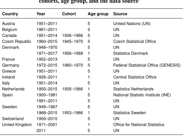
In order to quantify the scale, location, and variance of the first marriage using the de-composition method, we used population counts by sex, age, and marital status. Coale and McNeil (1972) applied their parametric model to cohort data, and other researchers, such as Goldstein and Kenney (2001) and Kaneko (2003) used cohort data for their analy-ses. However, other studies applied the CM model to period data as well (Rodr´ıguez and Trussell 1980; Peristera and Kostaki 2015), with the purpose of examining the current trends. It is well known that period and cohort data have strengths and weaknesses. The period data can describe current trends, while it mixes behaviours of different cohorts. The cohort data avoids the tempo distortions; however, birth cohorts only refer to one group of people present at a given time. Taking into consideration those advantages and disadvantages, in this study, we present results from both period and cohort data.

(12)

was built for six countries out of 15 countries in Table 1. When a single age group was available, the cohort data was reconstructed from the period data incrementing over age and time: for example, age 15 in 1940, age 16 in 1941, and so forth. Similarly, when the age group was five years, we used increments of five-year age groups every five calendar years: for example, ages 15–19 in 1960, ages 20–24 in 1965, and so forth. Only com-pleted cohorts that contained data until age 49 were selected. The information of cohort data can also be seen in Table 1.

Table 1: Countries included in the analysis, and analysed years, birth cohorts, age group, and the data source

Country Year Cohort Age group Source

Austria 1951–2011 5 United Nations (UN)

Belgium 1961–2011 5 UN

Canada 1951–2014 1936–1966 5 UN

Czech Republic 1960–2015 1945–1970 5 Czech Statistical Office

Denmark 1948–1970 5 UN

1971–2017 1956–1968 1 Statistics Denmark

France 1952–2013 5 UN

Germany 1972–2015 1960–1970 5 Federal Statistical Office (GENESIS)

Greece 1951–2011 5 UN

Ireland 1926–2011 1 Central Statistics Office

Italy 1951–2014 5 UN

Netherlands 1950–2015 1935–1966 1 Statistics Netherlands

Spain 1900–1981 5 National Statistic Institute (INE)

1991–2011 5 UN

Sweden 1949–1967 5 UN

1968–2015 1953–1966 1 Statistics Sweden

Switzerland 1950–2015 5 UN

United Kingdom 1971–2001 1 Office for National Statistics

2011 5 UN

Source: Czech Republic: population and housing census (www.czso.cz/csu/czso/home). Denmark: population register (www.statbank.dk). Germany: microcensus (www-genesis.destatis.de/genesis/online). Ireland: decennial census (www.cso.ie/en/databases). The Netherlands: population register (opendata.cbs.nl/dataportaal#/CBS/nl/). Spain: decennial census (www.ine.es/en/welcome.shtml). Sweden: population register (www.scb.se). The UK: estimation from decennial census (www.ons.gov.uk). UN (data.un.org).

3. Illustration of EYEM

3.1 The results of period data

(13)

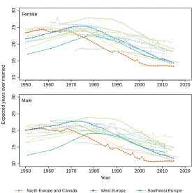
Figure 3: Time trends in period expected years ever married in 15 countries

1950 1960 1970 1980 1990 2000 2010 2020

10 15 20 25 30 ●●●●●●●●●●●●●●●●●●●●●●●●●●●●●●●●●●● ●●● ●●●●●●●● ● ●●●●●●●● ●● ●●●●●●●●● ● ● ● ● ●● ● ● ● ● ● ● ● ● ● ●●●●●● ●●●● ● ● ●●●● ●● ●●● ● ● ●● ● ● ●●●●●●●●●●●●●●●● ● ● ● ● ●●●●●●●●● ●● ●●● ●● ●●●●● ● ●● ● ● ● ● ●● ● ● ● ●●●●●●●●● ●●●●●●●●●●●●●●●●●●●●●●●●●● ●●●● ● ●● ● ●●●●●●● ●●● ●●● ● ● ●● ●●● ● ●●●●●● ●●●●● ●● ● ● ● ●● ● ●●● ● ●●●●●● Female

1950 1960 1970 1980 1990 2000 2010 2020

10 15 20 25 30 Year ●●●●●●●●●●●●●●●●●●●●●●●●●●●●●●●● ●● ●● ●● ●●● ●●●● ● ●● ●●●●●●●● ●●●●●●●●●● ● ● ● ● ●● ● ● ● ● ● ● ● ● ● ●●●●●● ●●●● ● ●●● ●● ●● ●●● ● ● ●● ● ● ●●●●●●●●●●●●●●●● ● ● ● ● ●●●●●●●●●●●●●● ●● ●●● ●● ●● ● ●● ● ●● ●● ● ● ●●●●●●●●● ●●●●●●●●●●●●●●●●●●●●●●●●●●●●●●● ●●● ●●●● ●●● ●●●●●●● ● ●● ●●● ● ●●●●●● ●●●●●●●● ● ● ●● ● ● ●● ● ●●●●●● Male

North Europe and Canada ● _{West Europe} _{Southeast Europe}

Expected y

ears e

v

er marr

ied

Note: North Europe and Canada comprise Canada, Denmark, and Sweden (highlighted). West Europe includes Austria, Belgium, France, Germany, the Netherlands (highlighted), Switzerland, and the UK. Southeast Europe represents the Czech Republic, Greece, Ireland (highlighted), Italy, and Spain.

Source: Authors’ calculations, using data described in Table 1.

(14)

example, in recent years, females from Denmark, France, Germany, Ireland, the Nether-lands, and Sweden have less than 15 years of period EYEM, while the other countries have more than 17 years. As seen in Figure 3, period EYEM started decreasing in the 1970s. Hence, we decompose period EYEM from 1970, and the results are presented in Figure 4.

Figure 4: Decomposition of the change over time in female period expected years ever married in 15 countries

−1.0 −0.5 0.0 0.5 1.0

1974 1979 1983 1988 1993 1999 2004 2008

Ireland −1.0 −0.5 0.0 0.5 1.0

1972 1977 1982 1987 1992 1997 2002 2007 2012

Netherlands −1.0 −0.5 0.0 0.5 1.0

1972 1977 1982 1987 1992 1997 2002 2007 2012

Sweden Scale Location Variance −2 −1 0 1 2

1975 1986 1996 2006 2013

Belgium −2 −1 0 1 2

1972 1977 1982 1987 1992 1997 2002 2007 2012

Denmark −2 −1 0 1 2

1973 1977 1982 1987 1992 1997 2002 2007 2012

Germany −2 −1 0 1 2

1972 1977 1986 1996 2006 2013

Greece −2 −1 0 1 2

1976 1990 2003 2008 2012

Italy −2 −1 0 1 2

1975 1986 1996 2006 2013

Spain −2 −1 0 1 2

1975 1983 1988 1992 1997 2002 2008 2013

Switzerland −2 −1 0 1 2

1973 1977 1982 1987 1992 1997 2005 2013

United Kingdom −4 −2 0 2 4

1972 1977 1985 1996 2006 2013

Austria −4 −2 0 2 4

1973 1978 1982 1987 1992 1997 2002 2008

Canada −4 −2 0 2 4

1972 1977 1982 1987 1992 1997 2002 2007 2012

Czech Republic −4 −2 0 2 4

1972 1977 1982 1987 1995 2002 2007 2012

France

Year

Contri

b

utions to change in the e

xpected y

ears e

v

er married

Note: The year presented corresponds to the mid-year between two points in times. For example, for the changes in period EYEM from 1970 to 1975, it is written as 1972. Details can be found in Appendix D.

(15)

Overall, location is the most influential factor in the changes in period EYEM. This shows that delayed marriage is the main contributor to nuptiality changes in most coun-tries and periods. The scale factor also has an important role in the changes in period EYEM. Sweden had a negative effect (contributing to the decline) of the scale compo-nent from 1985; later, Denmark, France, Germany, and Switzerland had it from 1990, the Netherlands from 1995, and Italy and the UK from 2000. A negative effect of the scale factor means that the decline in proportion of marriages contributed to the decline in pe-riod EYEM. In Sweden, the decline of pepe-riod EYEM is 28.1% due to nonmarriage and

71.9% due to delayed marriage from 1990 to 1995.5 _{However, it reversed from 2000 to}

2005, when nonmarriage contributed 82.8% to the decline of period EYEM and delayed marriage contributed 17.2% (see Table 2). In the period 2005 to 2010, the two compo-nents have opposing contributions. While most of the North and West European countries and Canada had negative scale and location effects, the scale factor has not started con-tributing enough to this decline in Austria, Belgium, Greece, and Spain. This shows that, in the latter group of countries, the main nuptiality change was delayed marriage. Lastly, the variance has not had much impact on the changes in period EYEM.

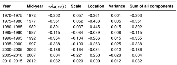
Table 2: Contribution of scale, location, and variance to the change in females’ period expected years ever married (35eM, 15(t)) in

Sweden, 1970 to 2015

Year Mid-year 35eM, 15(t) Scale Location Variance Sum of all components

1970–1975 1972 –0.302 0.057 –0.361 0.001 –0.303

1975–1980 1977 –0.351 0.052 –0.408 0.005 –0.351

1980–1985 1982 –0.391 0.037 –0.445 0.015 –0.392

1985–1990 1987 –0.115 –0.084 –0.039 0.008 –0.115

1990–1995 1992 –0.354 –0.104 –0.266 0.015 –0.355

1995–2000 1997 –0.338 –0.100 –0.263 0.025 –0.338

2000–2005 2002 –0.186 –0.164 –0.034 0.012 –0.186

2005–2010 2007 0.004 –0.221 0.253 –0.028 0.004

2010–2015 2012 –0.032 –0.020 0.000 –0.012 –0.032

Note: The sum of all components (scale, location, and variance) varies slightly from the difference in the expected years ever married (35eM, 15(t)), due to rounding the numbers to the third decimal point in the table.

Source: Authors’ calculations, using data described in Table 1.

However, caution is warranted in the interpretation of the results. Similar to pe-riod life expectancy, which corresponds to the mortality experience of a synthetic cohort, period EYEM is also an index combining the information of many cohorts. As previ-ous research has stated, a period index is biased by tempo effects (Winkler-Dworak and

5_{The percentages are calculated among negative values. For instance, the percentage of the contribution of}

scale from 1990 to 1995 (28.1%) is computed as0.104/(0.104 + 0.266).

.

(16)

Engelhardt 2004; Schoen and Canudas-Romo 2005; Bongaarts and Feeney 2006), and pe-riod EYEM could also be affected. Thus, the next section presents the changes in cohort EYEM over time.

3.2 The results of cohort data

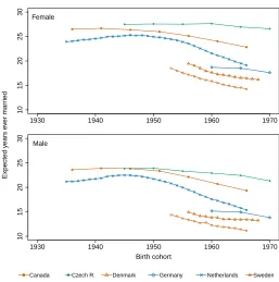
As the results for period data, the changes in cohort EYEM present similar trends for females and males (Figure 5). For all countries, males have smaller cohort EYEM, which means that males spend relatively longer periods in never married status. North Europe and Canada, which comprise Canada, Denmark, and Sweden, have a declining trend in all cohorts analysed. The Netherlands increased its cohort EYEM until the late 1940s birth cohort and decreased thereafter, while the Czech Republic shows an almost stagnating high EYEM trend.

Figure 5: Time trends in cohort expected years ever married in six countries

● ●

●● ●

●●● ●●●●●●

1930 1940 1950 1960 1970

10

15

20

25

30

● ● ● ●

● ●

Female

●● ●●●

●●

●●●●●●●

1930 1940 1950 1960 1970

10

15

20

25

30

Birth cohort

● ●

●

● Male

Canada ● Czech R. Denmark Germany Netherlands ● Sweden

Expected y

ears e

v

er marr

ied

(17)

(18)

Figure 6: Decomposition of the change over time in female cohort expected years ever married in six countries

−2.0 −1.5 −1.0 −0.5 0.0 0.5 1.0

1938 1943 1948 1953 1958 1963

Canada

−2.0 −1.5 −1.0 −0.5 0.0 0.5 1.0

1947 1952 1957 1962 1967

Czech Republic

−2.0 −1.5 −1.0 −0.5 0.0 0.5 1.0

1962 1967

Germany _Scale

Location Variance

−0.4 −0.2 0.0 0.2 0.4

1958 1963

Denmark

−0.4 −0.2 0.0 0.2 0.4

1937 1942 1947 1952 1957 1962

Netherlands

−0.4 −0.2 0.0 0.2 0.4

1957 1962

Sweden

Birth cohort

Contri

b

xpected y

ears e

v

er married

Note: The birth cohort presented corresponds to the mid-year between two points in birth cohorts. For example, for the changes in EYEM from 1950 to 1955, it is written as 1952. Details can be found in Appendix D.

(19)

4. Discussion and conclusion

Nonmarriage, delayed marriage, and expansion of first marriage timing are well reported and described as changes that happened in the second half of the 20th century (Lesthaeghe 1983; Van de Kaa 1987; Winkler-Dworak and Engelhardt 2004; Elzinga and Liefbroer 2007; European Commission 2015). In this article, we used the expected years ever mar-ried (EYEM) as a new alternative index to quantify nuptiality change and propose its decomposition into the three aforementioned components. Examining both period and cohort data allows us to study the changes in EYEM from both complementary perspec-tives. Period EYEM decreased from 1970, and the trends of changes of period EYEM are similar for males and females in the studied countries. Our results suggest that, in most countries and time periods, the decline in period EYEM is mainly due to delayed marriage. This result is consistent with other research that has analysed the US trend (Oppenheimer 1994; Goldstein and Kenney 2001). However, new trends can be seen in our selected countries, with the nonmarriage component influencing recently in Northern Europe, Canada, and in most West European countries. The expansion effect has prac-tically no influence on the changes in EYEM. Similar to the period EYEM trends, the trends of males’ cohort EYEM are similar to those observed for females, but with dif-ferent scales. The decline of the current cohort EYEM in Canada, Denmark, Germany, and the Netherlands is mainly due to delayed marriage, while nonmarriage was the main factor in Canada and the Netherlands in older cohorts. On the other hand, nonmarriage influenced just over half of the changes in cohort EYEM of Sweden.

(20)

to the Coale–McNeil model. This issue is particularly seen in some countries and times when the population consists of subpopulations whose first marriage timings are distinctly different from each other (Kaneko 2003; Peristera and Kostaki 2015). However, if data for those subpopulations were available, our decomposition method could be extended to also cover these cases. Hence, subpopulation analysis could increase the preciseness of nuptiality modeling, and future research might benefit from looking at the effects of scale, location, and variance on the changes in EYEM by subpopulations.

Finally, EYEM measures the expected number of years after first marriage. There-fore, it does not take into account exits from marriage (i.e., divorce/separation, widow-hood, or death). This study, however, focuses on the transition from never married to ever married status. For this reason, we introduced EYEM as an alternative index to study nuptiality changes. If the interest is to quantify the duration of first marriage until di-vorce, widowhood, or death, such as seen in Schoen and Nelson (1974) and Philipov and Jasilioniene (2008), one must consider exits from first marriage.

Which of the three effects, nonmarriage, delayed marriage, or expansion, has the most impact on nuptiality changes? How does the most influential factor differ by time periods, birth cohort, and countries? This study approaches those questions by intro-ducing a new index and decomposing its change into the contribution of each of those three components. By examining both period and cohort data, we present a full view of the changes in first marriage behaviours through Europe and Canada. The decomposi-tion steps presented in equadecomposi-tions (1) to (7) offer an open possibility for more elaborated parametric marriage models. Nuptiality dynamics keep evolving, and researchers would benefit from analysing future changes by using the methods developed here.

5. Acknowledgements

We are thankful to European Doctoral School of Demography (EDSD) and all the mem-bers of the cohort 2016–2017 for their helpful feedback and support. We appreciate also

the two anonymous reviewers and the editor ofDemographic Researchfor their

(21)

References

Andersen, P.K., Canudas-Romo, V., and Keiding, N. (2013). Cause-specific measures

of life years lost. Demographic Research29(41): 1127–1152. doi:10.4054/DemRes.

2013.29.41.

Becker, G.S. (1981).A treatise on the family. Cambridge: Harvard University Press.

Bergeron-Boucher, M.P., Ebeling, M., and Canudas-Romo, V. (2015). Decomposing

changes in life expectancy: Compression versus shifting mortality. Demographic

Re-search33(14): 391–424.doi:10.4054/DemRes.2015.33.14.

Bloom, D.E. and Bennett, N.G. (1990). Modeling American marriage patterns. Journal

of the American Statistical Association85(412): 1009–1017. doi:10.1080/01621459. 1990.10474971.

Blossfeld, H.P., Klijzing, E., Mills, M., and Kurz, K. (2005). Globalization, uncertainty

and youth in society. London: Routledge.doi:10.4324/9780203003206.

Bongaarts, J. and Feeney, G. (2006). The quantum and tempo of life-cycle events.Vienna

Yearbook of Population Research4: 115–151.

Coale, A.J. and McNeil, D.R. (1972). The distribution by age of the frequency of first

marriage in a female cohort. Journal of the American Statistical Association67(340):

743–749.doi:10.1080/01621459.1972.10481287.

Elzinga, C.H. and Liefbroer, A.C. (2007). De-standardization of family-life trajectories of

young adults: A cross-national comparison using sequence analysis.European Journal

of Population23(3): 225–250. doi:10.1007/s10680-007-9133-7.

European Commission (2015). Short analytical web note. Luxembourg: Publications Office of the European Union (Demography report 3/2015).

Goldstein, J.R. and Kenney, C.T. (2001). Marriage delayed or marriage forgone? New

co-hort forecasts of first marriage for U.S. women. American Sociological Review66(4):

506–519.

Kaneko, R. (2003). Elaboration of the Coale–McNeil nuptiality model as the generalized

log gamma distribution: A new identity and empirical enhancements. Demographic

Research9(10): 223–262.doi:10.4054/DemRes.2003.9.10.

Lesthaeghe, R. (1983). A century of demographic and cultural change in Western Europe:

An exploration of underlying dimensions. Population and Development Review9(3):

411–435.

Oppenheimer, V.K. (1988). A theory of marriage timing.American Journal of Sociology

(22)

Oppenheimer, V.K. (1994). Women’s rising employment and the future of the family in

industrial societies. Population and Development Review20(2): 293–342.

Perelli-Harris, B. (2014). How similar are cohabiting and married parents? Second

con-ception risks by union type in the United States and across Europe. European Journal

of Population30(4): 437–464. doi:10.1007/s10680-014-9320-2.

Peristera, P. and Kostaki, A. (2015). A parametric model for estimating nuptiality patterns

in modern populations. Canadian Studies in Population42(1): 130–148.

Philipov, D. and Jasilioniene, A. (2008). Union formation and fertility in Bulgaria and

Russia: A life table description of recent trends.Demographic Research19(62): 2057–

2114.doi:10.4054/DemRes.2008.19.62.

Preston, S., Heuveline, P., and Guillot, M. (2001). Demography: Measuring and

model-ing population processes. Oxford: Blackwell.

Rodr´ıguez, G. and Trussell, J. (1980). Maximum likelihood estimation of the parame-ters of Coale’s model nuptiality schedule from survey data. Voorburg: International Statistical Institute (World Fertility Survey technical bulletins 7).

Schoen, R. and Canudas-Romo, V. (2005). Timing effects on first marriage:

Twentieth-century experience in England and Wales and the USA. Population Studies59(2):

135–146.doi:10.1080/00324720500099124.

Schoen, R. and Nelson, V.E. (1974). Marriage, divorce, and mortality: A life table

analysis.Demography11(2): 267–290.doi:10.2307/2060563.

United Nations (2016). Demographic yearbook 2015. New York: Department of

Eco-nomic and Social Affairs (DESA) of the United Nations.

Van de Kaa, D.J. (1987). Europe’s second demographic transition. Population Bulletin

42(1): 1–59.

Vaupel, J.W. and Canudas-Romo, V. (2003). Decomposing change in life expectancy: A

bouquet of formulas in honor of Nathan Keyfitz’s 90th birthday. Demography40(2):

201–216.

Winkler-Dworak, M. and Engelhardt, H. (2004). On the tempo and quantum of first

marriages in Austria, Germany, and Switzerland: Changes in mean and variance.

De-mographic Research10(9): 231–264.doi:10.4054/DemRes.2004.10.9.

Wu, L.L. (2003). Event history models for life course analysis. In: Mortimer, J.T. and

(23)

Appendix A: The comparison between the observed and the

estimated age-specific first marriage rate

As Kaneko (2003) and Peristera and Kostaki (2015) pointed out, the CM model may not fit well to some countries and some time periods. If the CM model can not capture the observed rate, the presented results will be misleading. Thus, we compared the observed age-specific first marriage rate with the estimated one. The CM model generally estimates quite well to our selected data, especially countries that have single age groups, even though the CM model tends to underestimate the maximum value. For the countries that do not have single age data, the CM model does not fit as well as for the other countries. As Figure A-1 and A-2 show, the estimated rates have only slightly different scale and location from the observed data, which would not make our conclusion deviate from the findings presented here. Furthermore, as mentioned earlier in the main text, our methodology can adapt to other parametric formulations of the age patterns of marriage.

Figure A-1: Comparison between females’ observed and estimated period age-specific first marriage rates for Sweden

a) Year 1970

● ●● ● ● ● ● ● ● ● ● ● ● ● ● ●_● ● ● ● ● ● ● ● ●_{● ●}● ● ● ●●● ●●

15 20 25 30 35 40 45 50

0.00 0.02 0.04 0.06 0.08 0.10 0.12 Age

Age-specific first marr

iage rate

● Observed Estimated

b) Year 2015

● ● ● ● ● ● ● ● ● ● ● ● ● ● ● ● ● ● ● ● ● ● ● ● ● ● ● ● ● ●● ● ● ● ●

15 20 25 30 35 40 45 50

0.00 0.01 0.02 0.03 0.04 0.05 Age

iage rate

(24)

Figure A-2: Comparison between females’ observed and estimated cohort age-specific first marriage rates for Sweden

a) 1960 birth cohort

● ●● ● ● ● ● ● ● ● ● ●●● ● ● ● ● ● ● ●_● ● ●● ● ● ● ● ● ● ● ● ● ●

15 20 25 30 35 40 45 50

0.00 0.02 0.04 0.06 0.08 Age

iage rate

b) 1965 birth cohort

● ●● ● ● ● ● ● ● ● ● ● ● ● ● ● ● ● ● ● ● ● ●_{● ●}● ● ● ● ● ● ● ●_● ●

15 20 25 30 35 40 45 50

0.00

0.02

0.04

0.06

Age

iage rate

Note: There is a heap because cohort data is constructed from period data without smoothing.

Source: Authors’ calculations using data described in Table 1 of the main text.

Appendix B: Calculation process: Expected years ever married

We denote35eM, 15(t)as the expected years ever married from age 15 to age 50. It is

formulated as:

35eM, 15(t) =

Z 50

15

(1−lx,t)dx

=

Z 50

15

Fx,tdx, (8)

wherelxis a probability of remaining never married andFxis its cumulative probability

function. We use Rodr´ıguez and Trussell’s (1980) parametrisation for the density func-tion:

fx,t = Ct

1 σt

a1exp

h

a2( x−µt

σt

+a3)−exp{−a4(

x−µt

σt

+a3)}

i (9)

fx,t = Ct

1 σt

f0( x−µt

σt

(25)

where the usual values for the constants area1= 1.281,a2 =−1.145,a3= 0.805, and

a4= 1.896.f0is the density function defined from equation (9) as

f0(x) =a1exp

h

a2(x+a3)−exp{−a4(x+a3)}

i

. (10)

Its cumulative density function is written as

Fx,t=CtF0( x−µt

σt

), (11)

and substituting equation (11) in equation (8) results in an expression of EYEM that depends on our three variables of interest (scale, location, and variance) as

35eM, 15(t) =

Z 50

15 CtF0(

x−µt

σt

)dx. (12)

To quantify the effects of scale, location, and variance in the changes of EYEM over time, the partial derivative respect to time of the probability distribution in equation (12) is studied. Let a dot on top of a variable denote its partial derivative respect to time. The

change over time in EYEM, or ,35e˙M, 15(t), is decomposed as:

35e˙M, 15(t) =

∂35eM, 15(t) ∂Ct

˙ Ct+

∂35eM, 15(t) ∂µt

˙ µt+

∂35eM, 15(t) ∂σt

˙

σt, (13)

where each term is the change in35e˙M, 15(t)resulting from changes in the scale, location,

and variance respectively.

The derivative ofF0(x−_σµt

t )with respect to timetis

˙ F0(

x−µt

σt

) = f0(

x−µt

σt

)(

d

dt(x−µt)σt−(x−µt) ˙σt

σ2

t

)

= −1

σt

f0( x−µt

σt

) ˙µt−f0(

x−µt

σt

)(x−µt)

σ2

t

˙ σt;

substituting this in equation (12) helps obtaining the time derivative of EYEM as

35e˙M, 15(t) = ˙Ct

Z 50

15 F0(

x−µt

σt

)dx −µ˙t

Z 50

15 Ct

1 σt

f0( x−µt

σt

)dx

−σ˙t

Z 50

15 Ctf0(

x−µt

σt

)x−µt

σ2

t

(26)

Therefore, the changes of each factor is expressed as

∂35eM, 15(t) ∂Ct

˙ Ct= ˙Ct

Z 50

15 F0(

x−µt

σt

)dx (15)

for declines (increases) in the proportion ever marrying, or scale effect which contributes to the decline (increase) in the overall EYEM. The second term is

∂35eM, 15(t) ∂µt

˙

µt = −µ˙t

Z 50

15 Ct

1 σt

f0( x−µt

σt

)dx

= −µ˙t[F50,t−F15,t]

= −µ˙tF50,t

= −µ˙tCt, (16)

corresponding to the changes in the mean age at first marriage between ages 15 and 50. For all the cases when the mean age at first marriage has been increasing over time this term contributes negatively to the overall change in EYEM. Finally, the contribution of the standard deviation term is

∂35eM, 15(t) ∂σt

˙

σt = −σ˙t

Z 50

15 Ctf0(

x−µt

σt

)x−µt

σ2

t

dx

= −σ˙t

Z 50

15 fx,t

x−µt

σt

dx, (17)

which has negligible contribution in the cases studied here and presented in Tables 2 to A-3.

Appendix C: The decomposition to discrete data

The three parameters offxare estimated using Maximum Likelihood Estimation method

as suggested by Rodr´ıguez and Trussell (1980).

lnLH =

50

X

15

(Marxlog[F(x+0.5)] + NMarxlog[1−F(x+0.5)]), (18)

where Marxis ever married population at agexand NMarxis never married population

at agex, andFxis the cumulative probability function at agex. We checked the validity

(27)

on changing the single age groups to five-year age groups and showed that the parameters were still well estimated, although at different levels, but the time trends were preserved. Our assessment confirmed this and our results might be overestimated for the countries that have only five-year age groups (see Figure A-3 below). As age groups do not influ-ence the components’ time trends and their relative contribution to change in EYEM, it is likely that age group did not affect our overall conclusions.

Figure A-3: Comparison between the decomposition results using single age groups and five-year age groups for Sweden

a) Single age-groups

−0.4 −0.2 0.0 0.2 0.4

1972 1977 1982 1987 1992 1997 2002 2007 2012

Scale Location Variance

Year

Contributions to change in the e

xpected y

ears e

v

er marri

ed

b) Five year age-groups

−2 −1 0 1 2

1972 1977 1982 1987 1992 1997 2002 2007 2012

Scale Location Variance

Year

Contributions to change in the e

xpected y

ears e

v

er marri

ed

We followed Vaupel and Canudas-Romo (2003) of applying the continuous decom-position equation to discrete time data. To apply our decomdecom-position method to discrete time data, each function is estimated at their midpoint over a time interval (Preston, Heuveline, and Guillot 2001). For the functions except EYEM, an exponential change assumption is used.

υ_x_,_t₊h

2 =υx,t( υx,t+h

υx,t

)0.5 (19)

The derivative of the functionυ_x_,_t₊h

2 was estimated by

˙ υ_x_,_t₊h

2 =υx,t+h2(

log[υx,t+h

υx,t ]

(28)

EYEM was assumed to have a linear change in the interval and its midpoint was calculated as

υ_x_,_t₊h

2 =

υx,t+h+υx,t

2 (21)

and

˙ υ_x_,_t₊h

2 =

υx,t+h−υx,t

(29)

Appendix D: The results of decomposition for males

Figure A-4: Decomposition of the change over time in the male period expected years ever married in 15 countries

−1.0 −0.5 0.0 0.5 1.0

1972 1977 1982 1987 1992 1997 2002 2007 2012

Denmark −1.0 −0.5 0.0 0.5 1.0

1974 1979 1983 1988 1993 1999 2004 2008

Ireland −1.0 −0.5 0.0 0.5 1.0

1972 1977 1982 1987 1992 1997 2002 2007 2012

Netherlands −1.0 −0.5 0.0 0.5 1.0

1972 1977 1982 1987 1992 1997 2002 2007 2012

Sweden −2 −1 0 1 2

1973 1977 1982 1987 1992 1997 2002 2007 2012

Germany −2 −1 0 1 2

1972 1977 1986 1996 2006 2013

Greece −2 −1 0 1 2

1976 1990 2003 2008 2012

Italy −2 −1 0 1 2

1973 1977 1982 1987 1992 1997 2005 2013

United Kingdom −4 −2 0 2 4

1972 1977 1985 1996 2006 2013

Austria −4 −2 0 2 4

1975 1986 1996 2006 2013

Belgium −4 −2 0 2 4

1973 1978 1982 1987 1992 1997 2002 2008

Canada −4 −2 0 2 4

1972 1977 1982 1987 1992 1997 2002 2007 2012

Czech Republic −4 −2 0 2 4

1972 1977 1982 1987 1995 2002 2007 2012

France −4 −2 0 2 4

1975 1986 1996 2006 2013

Spain −4 −2 0 2 4

1975 1983 1988 1992 1997 2002 2008 2013

Switzerland Scale Location Variance Year Contri b

xpected y

ears e

v

er married

Note: The year presented corresponds to the mid-year between two times. For example, for the changes in period EYEM from 1970 to 1975, it is written as 1972. The details can be seen in Table A-1 in this supplemental material.

(30)

Table A-1: The contribution of each component to the time change in the female period expected years ever married

Country Year Mid-year Scale Location Variance

Austria 1970–1975 1972 0.429 –0.364 0.000

1975–1980 1977 –0.030 –1.153 0.005

1980–1991 1985 0.208 –1.222 0.021

1991–2001 1996 –0.156 –0.004 0.005

2001–2011 2006 –0.018 –2.518 0.165

2011–2015 2013 0.000 0.000 0.000

Belgium 1970–1981 1975 –0.030 –0.444 0.001

1981–1991 1986 –0.123 –1.315 0.011

1991–2001 1996 –0.045 –1.739 0.051

2001–2011 2006 0.109 –1.827 0.245

2011–2015 2013 0.000 0.000 0.000

Canada 1971–1976 1973 0.083 –0.252 0.000

1976–1980 1978 –0.064 –1.449 0.004

1980–1985 1982 –0.143 –0.578 0.008

1985–1990 1987 –0.201 –1.401 0.004

1990–1995 1992 –0.215 –1.019 0.015

1995–2000 1997 –0.295 –0.022 0.054

2000–2005 2002 –0.619 –3.850 0.130

2005–2011 2008 0.224 2.816 –0.114

Czech Republic 1970–1975 1972 0.168 0.059 0.000

1975–1980 1977 0.107 0.032 0.000

1980–1985 1982 –0.416 –0.431 0.000

1985–1990 1987 –0.128 –0.107 0.000

1990–1995 1992 –0.792 –1.965 0.005

1995–2000 1997 –0.127 –2.671 0.017

2000–2005 2002 0.272 –2.363 0.031

2005–2010 2007 0.263 –2.575 0.131

2010–2015 2012 0.270 –2.596 0.311

Denmark 1970–1975 1972 –0.169 –1.447 0.005

1975–1980 1977 0.023 –0.385 0.001

1980–1985 1982 0.058 –0.511 0.006

1985–1990 1987 0.053 –0.420 0.022

1990–1995 1992 –0.096 –0.205 0.013

1995–2000 1997 –0.221 0.025 –0.005

2000–2005 2002 –0.199 0.050 –0.017

2005–2010 2007 0.063 –0.006 –0.005

2010–2015 2012 –0.001 –0.203 0.008

France 1970–1975 1972 0.046 –0.410 0.001

1975–1980 1977 0.172 0.147 0.001

1980–1985 1982 –0.111 –1.645 0.012

1985–1990 1987 0.065 –3.139 0.051

1990–2000 1995 –0.184 –1.226 0.068

2000–2005 2002 –0.300 –1.325 0.263

2005–2010 2007 –0.991 –0.327 –0.061

(31)

Table A-1: (Continued)

Germany 1972–1975 1973 0.002 –1.054 0.002

1975–1980 1977 0.134 –1.514 0.007

1980–1985 1982 0.184 –1.503 0.017

1985–1990 1987 0.205 –1.389 0.037

1990–1995 1992 –0.122 –0.657 0.018

1995–2000 1997 –0.181 –1.154 0.053

2000–2005 2002 –0.184 –1.255 0.077

2005–2010 2007 –0.342 –1.067 0.055

2010–2015 2012 –0.389 –0.530 0.042

Greece 1970–1975 1972 0.000 0.000 0.000

1975–1980 1977 0.000 0.000 0.000

1981–1991 1986 0.256 –0.997 –0.006

1991–2001 1996 0.117 –1.420 0.035

2001–2011 2006 0.055 –1.363 0.075

2011–2015 2013 0.000 0.000 0.000

Ireland 1971–1977 1974 0.242 0.012 0.000

1977–1981 1979 0.047 –0.042 0.000

1981–1986 1983 0.071 –0.243 0.000

1986–1991 1988 0.036 –0.246 0.001

1991–1996 1993 0.011 –0.363 0.003

1996–2002 1999 0.048 –0.467 0.015

2002–2006 2004 0.013 –0.214 0.024

2006–2011 2008 –0.100 –0.071 0.008

2011–2015 2013 0.000 0.000 0.000

Italy 1971–1981 1976 0.471 –0.294 0.001

1981–2000 1990 0.095 –1.276 0.026

2000–2006 2003 –0.140 –1.316 0.098

2006–2010 2008 –0.391 –0.838 0.077

2010–2014 2012 –0.465 –0.951 0.024

Netherlands 1970–1975 1972 0.042 0.037 0.000

1975–1980 1977 0.051 –0.217 0.000

1980–1985 1982 0.038 –0.334 0.001

1985–1990 1987 0.033 –0.345 0.004

1990–1995 1992 –0.026 –0.276 0.005

1995–2000 1997 –0.058 –0.266 0.008

2000–2005 2002 –0.067 –0.257 0.017

2005–2010 2007 –0.096 –0.175 0.007

2010–2015 2012 –0.163 –0.098 0.002

Spain 1970–1981 1975 0.310 0.120 0.001

1981–1991 1986 0.206 –1.412 0.022

1991–2001 1996 0.087 –1.815 0.058

2001–2011 2006 0.175 –1.385 0.250

2011–2015 2013 0.000 0.000 0.000

Sweden 1970–1975 1972 0.057 –0.361 0.001

1975–1980 1977 0.052 –0.408 0.005

1980–1985 1982 0.037 –0.445 0.015

1985–1990 1987 –0.084 –0.039 0.008

1990–1995 1992 –0.104 –0.266 0.015

1995–2000 1997 –0.100 –0.263 0.025

2000–2005 2002 –0.164 –0.034 0.012

2005–2010 2007 –0.221 0.253 –0.028

(32)

Switzerland 1970–1980 1975 0.247 –1.174 0.010

1980–1986 1983 0.129 –0.991 0.018

1986–1990 1988 0.054 –0.493 0.038

1990–1995 1992 –0.051 –0.648 0.023

1995–2000 1997 –0.066 –0.850 0.043

2000–2005 2002 0.041 –1.540 0.092

2005–2011 2008 –0.276 –0.451 0.025

2011–2015 2013 –0.190 –0.540 0.022

United Kingdom 1971–1975 1973 0.057 –0.050 0.000

1975–1980 1977 0.044 –0.205 0.000

1980–1985 1982 0.041 –0.357 0.001

1985–1990 1987 0.016 –0.288 0.003

1990–1995 1992 –0.006 –0.313 0.005

1995–2000 1997 –0.001 –0.404 0.017

2000–2011 2005 –0.538 –0.659 0.037

2011–2015 2013 0.000 0.000 0.000

Table A-2: The contribution of each component to the time change in the male period expected years ever married

Austria 1970–1975 1972 –0.173 0.039 –0.006

1975–1980 1977 –0.076 –0.874 0.021

1980–1991 1985 0.157 –0.972 0.043

1991–2001 1996 –0.103 –0.258 0.042

2001–2011 2006 –0.034 –2.513 0.307

2011–2015 2013 0.000 0.000 0.000

Belgium 1970–1981 1975 0.073 –0.362 0.002

1981–1991 1986 0.111 –1.199 0.015

1991–2001 1996 –0.056 –1.731 0.076

2001–2011 2006 0.511 –2.487 0.598

2011–2015 2013 0.000 0.000 0.000

Canada 1971–1976 1973 0.305 –0.132 0.004

1976–1980 1978 0.241 –1.458 0.009

1980–1985 1982 0.090 –0.651 0.029

1985–1990 1987 0.000 –1.374 –0.011

1990–1995 1992 –0.232 –1.220 0.049

1995–2000 1997 –0.411 –0.350 0.156

2000–2005 2002 –0.694 –3.497 0.188

2005–2011 2008 0.082 3.318 –0.227

(33)

Czech Republic 1970–1975 1972 0.140 –0.003 0.001

1975–1980 1977 –0.110 –0.278 0.002

1980–1985 1982 0.020 –0.429 0.008

1985–1990 1987 –0.205 0.143 0.001

1990–1995 1992 –0.153 –1.356 0.009

1995–2000 1997 0.070 –1.894 0.005

2000–2005 2002 0.161 –2.540 0.077

2005–2010 2007 0.437 –2.764 0.214

2010–2015 2012 0.368 –3.024 0.558

Denmark 1970–1975 1972 0.463 –0.995 –0.001

1975–1980 1977 0.033 –0.411 0.003

1980–1985 1982 0.089 –0.539 0.016

1985–1990 1987 0.078 –0.455 0.047

1990–1995 1992 –0.164 –0.107 0.007

1995–2000 1997 –0.255 0.098 –0.018

2000–2005 2002 –0.177 0.072 –0.023

2005–2010 2007 0.091 –0.013 –0.002

2010–2015 2012 0.016 –0.182 0.012

France 1970–1975 1972 0.102 –0.036 –0.009

1975–1980 1977 0.147 0.097 0.003

1980–1985 1982 0.457 –1.399 0.008

1985–1990 1987 0.329 –3.135 0.090

1990–2000 1995 –0.309 –1.130 0.081

2000–2005 2002 –0.338 –1.292 0.291

2005–2010 2007 –0.930 –0.225 –0.068

2010–2015 2012 0.000 0.000 0.000

Germany 1972–1975 1973 –0.102 –0.590 0.010

1975–1980 1977 0.039 –1.243 0.029

1980–1985 1982 –0.158 –1.134 0.032

1985–1990 1987 0.066 –1.301 0.066

1990–1995 1992 0.062 –0.990 0.080

1995–2000 1997 –0.299 –1.113 0.077

2000–2005 2002 –0.210 –1.346 0.132

2005–2010 2007 –0.624 –0.624 0.023

2010–2015 2012 –0.404 –0.216 0.010

Greece 1970–1975 1972 0.000 0.000 0.000

1975–1980 1977 0.000 0.000 0.000

1981–1991 1986 0.126 –1.002 0.039

1991–2001 1996 0.144 –1.454 0.165

2001–2011 2006 –0.061 –1.134 0.164

2011–2015 2013 0.000 0.000 0.000

Ireland 1971–1977 1974 0.332 0.039 0.000

1977–1981 1979 0.072 –0.033 0.000

1981–1986 1983 0.127 –0.212 0.000

1986–1991 1988 0.091 –0.240 0.001

1991–1996 1993 0.038 –0.351 0.005

1996–2002 1999 0.080 –0.422 0.016

2002–2006 2004 0.072 –0.242 0.038

2006–2011 2008 –0.081 –0.066 0.006

(34)

Italy 1971–1981 1976 0.249 –0.022 –0.001

1981–2000 1990 0.050 –1.136 0.040

2000–2006 2003 0.077 –1.769 0.226

2006–2010 2008 –0.234 –1.166 0.215

2010–2014 2012 –0.586 –0.777 0.053

Netherlands 1970–1975 1972 –0.025 0.028 0.000

1975–1980 1977 0.018 –0.232 0.000

1980–1985 1982 0.050 –0.325 0.002

1985–1990 1987 0.045 –0.359 0.008

1990–1995 1992 –0.041 –0.279 0.008

1995–2000 1997 –0.057 –0.291 0.013

2000–2005 2002 –0.042 –0.289 0.030

2005–2010 2007 –0.068 –0.199 0.025

2010–2015 2012 –0.217 0.011 –0.010

Spain 1970–1981 1975 –0.047 0.559 0.009

1981–1991 1986 0.273 –1.385 0.053

1991–2001 1996 0.022 –1.701 0.071

2001–2011 2006 0.459 –2.082 0.563

2011–2015 2013 0.000 0.000 0.000

Sweden 1970–1975 1972 0.083 –0.375 0.002

1975–1980 1977 0.096 –0.435 0.011

1980–1985 1982 0.088 –0.490 0.032

1985–1990 1987 –0.097 –0.024 0.012

1990–1995 1992 –0.135 –0.205 0.012

1995–2000 1997 –0.110 –0.221 0.024

2000–2005 2002 –0.137 –0.037 0.015

2005–2010 2007 –0.165 0.221 –0.027

2010–2015 2012 –0.021 0.043 –0.021

Switzerland 1970–1980 1975 0.230 –0.870 0.013

1980–1986 1983 0.020 –0.896 0.026

1986–1990 1988 –0.033 –0.686 0.079

1990–1995 1992 –0.023 –0.836 0.051

1995–2000 1997 0.127 –1.399 0.153

2000–2005 2002 0.110 –1.765 0.218

2005–2011 2008 –0.606 0.051 –0.041

2011–2015 2013 –0.351 –0.183 –0.031

United Kingdom 1971–1975 1973 0.038 –0.063 0.000

1975–1980 1977 0.032 –0.177 0.000

1980–1985 1982 0.035 –0.336 0.002

1985–1990 1987 0.028 –0.287 0.006

1990–1995 1992 –0.011 –0.291 0.007

1995–2000 1997 0.009 –0.399 0.025

2000–2011 2005 –0.423 –0.675 0.075

2011–2015 2013 0.000 0.000 0.000

(35)

Figure A-5: Decomposition of the change over time in the male cohort expected years ever married in six countries

−2.0 −1.5 −1.0 −0.5 0.0 0.5 1.0

1938 1943 1948 1953 1958 1963

Canada

−2.0 −1.5 −1.0 −0.5 0.0 0.5 1.0

1947 1952 1957 1962 1967

Czech Republic

−2.0 −1.5 −1.0 −0.5 0.0 0.5 1.0

1962 1967

Germany _Scale

Location Variance

−0.4 −0.2 0.0 0.2 0.4

1958 1963

Denmark

−0.4 −0.2 0.0 0.2 0.4

1937 1942 1947 1952 1957 1962

Netherlands

−0.4 −0.2 0.0 0.2 0.4

1957 1962

Sweden

Birth cohort

Contri

b

xpected y

ears e

v

er married

Note: The birth cohort presented corresponds to the mid-year between two birth cohorts. For example, for the changes in cohort EYEM from 1950 to 1955, it is written as 1952. Detailed information can be seen in Table A-1 in this supplemental material.

(36)

Table A-3: The contribution of each component to the time change in the cohort expected years ever married

Female Male

Country Year Mid-year Scale Location Variance Scale Location Variance

Canada 1936–1941 1938 0.130 0.327 0.000 0.070 0.363 –0.005

1941–1946 1943 –0.253 –0.178 0.000 –0.193 0.213 –0.003

1946–1951 1948 –0.318 0.097 0.000 –0.436 0.156 –0.001

1951–1956 1953 –0.706 –0.214 0.000 –0.600 –0.224 0.010

1956–1961 1958 –0.632 –0.992 –0.006 –0.230 –1.209 0.046

1961–1966 1963 0.155 –1.647 –0.029 0.191 –1.767 0.077

Czech Republic 1945–1950 1947 0.094 0.071 0.000 –0.175 0.327 –0.001

1950–1955 1952 –0.076 0.002 0.000 –0.255 –0.259 0.004