Annales
Geophysicae
Modelling interplanetary CMEs using magnetohydrodynamic
simulations
P. J. Cargill and J. M. Schmidt
Space and Atmospheric Physics The Blackett Laboratory Imperial College London SW7 2BW, UK Received: 9 October 2001 – Revised: 1 February 2002 – Accepted: 12 February 2002
Abstract. The dynamics of Interplanetary Coronal Mass Ejections (ICMEs) are discussed from the viewpoint of nu-merical modelling. Hydrodynamic models are shown to give a good zero-order picture of the plasma properties of ICMEs, but they cannot model the important magnetic field effects. Results from MHD simulations are shown for a number of cases of interest. It is demonstrated that the strong interac-tion of the ICME with the solar wind leads to the ICME and solar wind velocities being close to each other at 1 AU, de-spite their having very different speeds near the Sun. It is also pointed out that this interaction leads to a distortion of the ICME geometry, making cylindrical symmetry a dubi-ous assumption for the CME field at 1 AU. In the presence of a significant solar wind magnetic field, the magnetic fields of the ICME and solar wind can reconnect with each other, leading to an ICME that has solar wind-like field lines. This effect is especially important when an ICME with the right sense of rotation propagates down the heliospheric current sheet. It is also noted that a lack of knowledge of the coronal magnetic field makes such simulations of little use in space weather forecasts that require knowledge of the ICME mag-netic field strength.
Key words. Interplanetary physics (interplanetary magnetic fields) Solar physics, astrophysics, and astronomy (flares and mass ejections) Space plasma physics (numerical simulation studies)
1 Introduction
Coronal Mass Ejections (CMEs) are the most important so-lar cause of adverse space weather conditions. They can be defined as the expulsion of a large volume of plasma and associated magnetic field from the Sun’s gravitational field. CME masses can be as large as 1016g, and their velocities can lie anywhere between 100 and 2000 km/s (Hundhausen, 1999). It is clear that forces associated with the CME mag-Correspondence to: P. J. Cargill ([email protected])
netic field are responsible for their outward motion, although the precise cause of the eruption is not yet established (e.g. Chen, 2001; Klimchuk, 2001; Low, 2001).
There are two major reasons why CMEs and associated ICMEs lead to adverse space weather conditions. The first is that the magnetic field in an ICME is often very well orga-nized, leading to a sustained period (up to 12 h) of southward Interplanetary Magnetic Field (IMF) at the Earth (e.g. Tsu-rutani et al., 1988; Chen et al., 1997). This, in turn, leads to enhanced magnetic reconnection at the sub-solar magne-topause, with injection of energy into the magnetosphere, es-pecially the ring current. ICMEs are often also observed to be moving rapidly on their arrival at the Earth, leading to an en-hancement of the reconnection process. The second reason is that during their evolution in the inner solar wind, ICMEs are able to accelerate energetic protons very effectively, presum-ably at a shock wave driven ahead of the CME (e.g. Reames, 1999).
880 P. J. Cargill and J. M. Schmidt: Modelling interplanetary CMEs the problem of ICME propagation has received considerable
attention in recent years, motivated primarily by excellent in situ spacecraft observations both sunward of, and near the Earth, and in the more distant heliosphere. Section 2 of this paper summarizes the key observational points. Section 3 addresses the topic of ICME evolution from the viewpoint of hydrodynamic and magnetohydrodynamic (MHD) mod-els, and Sect. 4 presents a view of where this field ought to be going in the future.
2 The important issues that modelling needs to address
As we noted above, there are excellent in situ spacecraft observations of Interplanetary CMEs (ICMEs) in much of the heliosphere. The majority of the observations have been made just upstream of the Earth by a single spacecraft. In ad-dition, there are two other sparser sets of observations. One set is from the distant heliosphere (>4 AU) from the Ulysses mission and provides major constraints in our understand-ing of the radial evolution of ICMEs. The second set comes from multiple spacecraft. By necessity, these are serendipi-tous, but are important for understanding the 3-D structure of ICMEs. As we will show in Sect. 3, present-day models can address the first two of these issues.
2.1 Factors at 1 AU
ICMEs have been observed at 1 AU since the start of the space age, but it is only really in the past two decades that their true structure has been fully understood. The ma-jor data sets have been obtained from the IMP-8 (1973– present), ISEE-3 (1978–1982), WIND (1994–present) and ACE (1997–present) spacecraft. The ISEE-3 and ACE data sets are especially important since they were obtained from the L1 point, allowing continual solar wind coverage. While ICMEs come in a variety of forms, Burlaga et al. (1981) and Klein and Burlaga (1982) noted that a significant fraction of ICMEs had smooth magnetic field profiles that changed on time scales of hours, and lower than usual plasma tem-peratures. They named such ICMEs “magnetic clouds” and at least 30–40% of ICMEs are of this type (Gosling, 1990). Magnetic clouds are vast structures, often being 0.25 AU in diameter, and taking a day to pass by the Earth. From the viewpoint of space weather, their importance lies in the fact that the smoothly-changing magnetic field often leads to an IMF that is southward for many hours, with values often in excess of−20 nT. For this reason, the emphasis of the present paper is on magnetic clouds. Magnetic clouds have been interpreted as being large cylindrically symmetric magnetic flux ropes (Burlaga, 1988; Lepping et al., 1990) attached to the Sun at both ends, although multi-spacecraft observa-tions (see below) suggest that cylindrical symmetry is not a good assumption. Since it is unlikely that such organized flux ropes could form spontaneously from a turbulent solar wind, their origin must be solar. The most attractive picture is that the magnetic cloud originates as a large solar
loop-like structure, and is in fact the remnants of a coronal flux rope (often referred to as the prominence cavity: Low, 1996; Hundhausen, 1999), although flux ropes can also form due to a reconnection process that takes place during eruption (e.g. Gosling et al., 1995).
The structure of a magnetic cloud at 1 AU is determined by both its initial state, and by its interaction with the solar wind en route from the Sun. Indeed, the fact that an orga-nized structure like a magnetic cloud can survive to 1 AU suggests that it contains significant inherent robustness, and is stable to solar wind perturbations. However, the interac-tion of an ICME with the solar wind is an important factor in determining its properties at 1 AU. The clearest evidence that significant interaction does take place can be seen by a comparison of the distribution of observed CME speeds at the Sun, and those detected by spacecraft in the heliosphere. Gopalswamy et al. (2000) have carried out such a compari-son for 28 CMEs seen in the SOHO epoch, using data from the LASCO instrument and the ACE spacecraft, and show that while CMEs at the Sun cover a wide range of speeds (100–1500 km/s), at 1 AU the speeds are bunched between 350 and 550 km/s. (Note that most of the CMEs in this study were magnetic clouds.) Hence, the interaction between the ICME and the solar wind tends to bring their velocities closer together, with slow ICMEs being accelerated and fast ones being decelerated. Lindsay et al. (1999) have carried out a similar study using data from the SMM and Solwind coron-agraphs, and interplanetary data from Pioneer Venus Orbiter. They reached similar conclusions to Gopalswamy et al., but also note a positive correlation between the CME speed at the Sun and the maximum total field strength in the ICME (see also Owens and Cargill, 2002). However, they could es-tablish no real correlation between the southward IMF and ICME speed.
2.2 Factors at larger distances
Observations at different heliocentric distances permit one to study how ICMEs evolve as they move away from the Sun, and, hence, constrain theories pertaining to this evo-lution. Data obtained by the Voyager spacecraft established that clouds continue to expand beyond 1 AU (Burlaga and Behannon, 1982). The same is true for ICMEs seen out of the ecliptic plane, especially in regions of pure high-speed solar wind. In this regard, the Ulysses mission has provided a unique and probably unrepeatable data set. During 1993–98, the Ulysses spacecraft spent considerable time in regions of purely high-speed solar wind, only passing through regions of low-speed wind as it carried out its fast latitude scan in 1995. (The transition from high- to low-speed wind involved passage through an ICME, Forsyth et al., 1996). Ulysses detected a significant number of ICMEs in regions of high-speed wind, with detections being made at 54◦S, with many of these events being magnetic clouds, so that flux rope struc-tures must be able to survive to large distances.
ICME is characterized by a very low plasma density, and a relatively strong forward and reverse shock pair. (These are sometimes magnetic clouds, further evidence of the robust-ness of the magnetic flux rope in the solar wind.) An inter-pretation originally proposed by Gosling et al. (1994) was that these ICMEs were “overexpanding”, having begun life with a large excess of plasma pressure, which had expended its energy into creating the shock pairs. We will show that the overexpansion in fact plays a significant role in maintaining a magnetic cloud structure.
2.3 What multi-point observations tell us
Information concerning the multi-dimensional structure of ICMEs requires data from more than one spacecraft. While the models do not yet address these issues, we include this short summary for completeness. There are many cases where an ICME was observed by a spacecraft near the L1 point, and later on nearer to the Earth (ISEE-3 and IMP-8 are the best examples of such a conjunction). However, their very proximity, as well as close alignment along the Sun-Earth line rules out such observations as a major source of useful information about structures organized in the scales of ICMEs. One requires well-separated spacecraft, and such conjunctions are generally unplanned. The authors are aware of seven examples. Two involve the Ulysses spacecraft (Hammond et al., 1995; Gosling et al., 1995), four the NEAR spacecraft (Mulligan et al., 1999), and one Pioneer Venus Or-biter (Mulligan and Russell, 2001).
Hammond et al. (1995) reported observations of a mag-netic cloud by Ulysses (at 5 AU) and Geotail (at 1 AU), at a time when Ulysses was 20◦S and 50◦W of Geotail. The por-tion of the ICME seen by Ulysses was travelling much faster (200 km/s), but despite this, there are recognizable similari-ties in the magnetic field profiles. A picture is presented of an ICME with parts in both high- and low-speed wind, presum-ably with the part in the low speed wind being accelerated due to magnetic tension forces associated with the field line connection to the high-speed wind, although detailed mod-elling has not been carried out. A second event was reported by Gosling et al. (1995) using data from Ulysses (at 3.53 AU, and 54◦S) and IMP-8. At Ulysses, this was an overex-panding ICME (see previous section), with a forward-reverse shock pair, while at IMP-8 there was only a leading shock. The difference in the ICME appearance at each latitude must be due to differences in the interplanetary medium that each part of the ICME experiences. However, in this case, there was less similarity between the magnetic field profiles.
In 1997 when the Wind and NEAR spacecraft were sepa-rated by between 0.18 and 0.63 AU, and by between 1◦and 33◦in azimuth (Mulligan et al., 1999), four magnetic clouds were seen at a range of spacecraft separations. A limitation of the analysis is the absence of solar wind plasma measure-ments from NEAR (hence, the restriction to well-organized magnetic structures). When the spacecraft were close to-gether (0.18 AU and 1◦), the leading shock positions differed somewhat, but the major magnetic field structures were
read-ily recognizable in both data sets, though there were very no-ticeable differences. As the spacecraft separation increased, the differences became unmistakeable. For example, at a sep-aration of 0.28 AU and 5◦, the polarity of thex andz mag-netic field components in the ICME were different (where the x and zdirections were along the Earth-Sun line, and south-north, respectively), though the sense of field rotation appeared to be the same. The dissimilarities increased in the other two examples. In one case, although the sense of ro-tation was the same, the field components appear to be re-versed when NEAR and Wind are compared. In the final case, Wind saw two ICMEs, whereas NEAR saw only one. This case had the largest separation (0.63 AU and 33◦), so it is unclear whether the two spacecraft saw the same event. Further spacecraft conjunctions, as well as a modelling ef-fort, are greatly needed to resolve the issues raised here.
3 Results from numerical models
Despite the development of analytic models involving vari-ous degrees of approximation (e.g. Chen, 1996; Kumar and Rust, 1996; Vandas et al., 1993), it is numerical simulations that have shed the most light on the dynamics of ICMEs. We focus here on such simulations. ICMEs are usually modelled using the equations of magnetohydrodynamics (MHD):
∂ρ
∂t +∇·(ρV)=0 (1)
ρ∂V
∂t +ρ(V ·∇)V = −∇P +
J×B
c −ρ
GMs
r2 rˆ (2)
∂B
∂t −∇×(V×B)=0 (3)
∇·B=0 (4)
d dt
P
ργ
=0 (5)
in the usual notation where CGS/Gaussian units are used. Note that while ICMEs are technically a collisionless plasma, their large-scale makes them amenable to modelling using the MHD equations. Kinetic wave-particle interactions are likely to only be important at regions of strong current, such as magnetic reconnection sites.
882 P. J. Cargill and J. M. Schmidt: Modelling interplanetary CMEs
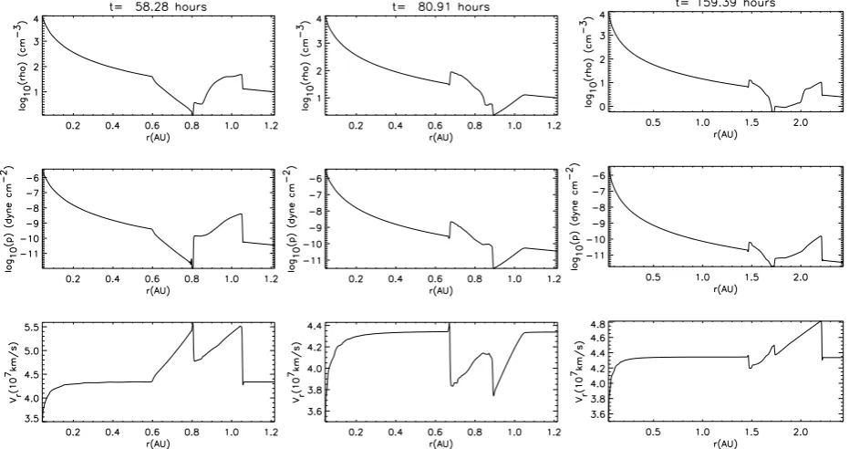
Fig. 1. Results from one-dimensional hydrodynamic ICME models. In Figs. 1a and 1b, results are shown when the ICME has reached approximately 1 AU (after 58 and 81 h, respectively), and in Fig. 1c when it is approaching 2 AU (after 159 h). In each case, the three panels show the density, pressure and radial velocity. The Fig. 1a (1b) case shows that the initial ICME speed is a factor of two bigger (smaller) than the solar wind speed, but the initial ICME density and pressure are the same as the solar wind. In Fig. 1c, the initial ICME pressure is a factor of 10 larger than that in the solar wind, but the density and radial velocity are the same.
1980). The best resolution of this problem involves solv-ing for the magnetic field on a mesh located at the edges of the computational cells (Evans and Hawley, 1988; DeVore, 1991), which ensures that is satisfied to machine accuracy. 3.1 Hydrodynamic models: a zero-order understanding of
ICME-related plasma flows
From the viewpoint of space weather, the magnetic field as-sociated with an ICME is the most important quantity that needs to be addressed in MHD models. However, it is clear that much useful information on the plasma flows and shock waves associated with ICMEs can be obtained from hydro-dynamic models (i.e. models with B = 0 in Eqs. 1–5). While not using explicit models of ICMEs, Hundhausen and Gentry (1968) demonstrated clearly the formation of shock waves in a spherically symmetric solar wind into which a density and/or velocity perturbation was introduced near the Sun. Gosling, Riley and collaborators have recently stud-ied overexpanding ICMEs using one-dimensional (Gosling et al., 1994; Gosling and Riley, 1996; Gosling et al., 1998) and two-dimensional (Riley et al., 1997) hydrodynamic sim-ulations. An example of the type of evolution that occurs is shown by the one-dimensional models presented in Figs. 1a– c. The model was run using our flux corrected transport (FCT) numerical scheme (Zalesak, 1979; Spicer, 1993). In Figs. 1a and b, the ICME evolution is followed from 10–
250RS with 600 grid points. The solar wind speed at the
inner boundary (located at 10RS) is 350 km/s, increasing to
430 km/s at 1 AU. The density at 1 AU is 10 cm−3. In Fig. 1a (1b), the ICME is modelled by increasing (decreasing) the solar wind speed by a factor of 2 in the region between 0.057 and 0.13 AU (i.e. 12.2–27RS). This models fast and slow
ICMEs.
The three panels in each figure show the density, pressure and velocity when the leading edge of the ICME has just passed 1 AU. When the ICME moves faster than the solar wind, the overall structure from right to left on the plots is as follows. First, there is a bow shock, compressing and ac-celerating the solar wind. Behind this is the residue of the initial velocity pulse, which terminates at an abrupt decrease of the pressure. Behind this is a rarefaction wave, as the trail-ing solar wind is sucked along behind the ICME. The ICME plasma structure is, therefore, the result of the interaction of these waves with the initial fast-moving plasma.
the ICME evolves, although the one-dimensional models will tend to overestimate the interaction with the solar wind.
As a final example of one-dimensional modelling, we show the evolution of an ICME whose initial pressure is high (factor of 10 larger than the solar wind), but is initially sta-tionary with respect to the wind. The simulation box is now 2.5 AU long, with 1200 grid points. In this case, the ini-tial ICME expands in both directions in order to relieve the overpressure, resulting in a pair of shock waves: a forward shock plows into the preceeding solar wind, and a reverse shock into the trailing wind, with the ICME being the region between the shocks. These are seen at 2.2 and 1.45 AU, re-spectively. Such classes of ICMEs have been studied in the context of observations from the Ulysses spacecraft of over-expanding ICMEs that have such a shock pair, as well as a low internal density which develops at larger distances. 3.2 MHD models
While hydrodynamic models can clearly shed important light on the flows induced in the solar wind by an ICME, they ob-viously cannot describe the magnetic field properties which are critical in determining the geoeffectiveness of a ICME. This requires the use of MHD codes. Before describing re-sults from such codes, it is important to note some problems that arise in attempting to model the evolution of an ICME. In our view, the major challenge is prescribing a suitable ini-tial magnetic field geometry such that (a) the solution is not dominated by spurious effects due to a lack of initial equi-librium and (b) the condition∇·B = 0 is satisfied. The latter can be dealt with by specifying a vector potential ev-erywhere in the simulation box so that∇·B=0 is satisfied trivially. However, problems arise when one tries to initialize a simulation with a magnetic flux rope embedded in a radial solar wind magnetic field. The solar wind field is distorted around the flux rope, and it is very quickly apparent that one cannot generally write down an analytic form of the vector potential for this situation, although special solutions do ex-ist (see Schmidt, 2000). A variety of approximate methods have also been proposed (e.g. Detman et al., 1991; Vandas et al., 1995).
In this section we focus on three aspects of the propagation of ICMEs in the solar wind:
(1) the plasma flows induced by the interaction of ICMEs with the solar wind,
(2) the survival of flux rope structures to large radial dis-tances, and
(3) magnetic reconnection between the ICME and solar wind magnetic fields.
All simulations shown are performed using 2.5 dimensional FCT codes in either Cartesian or spherical geometries (see Cargill et al., 1995; 1996; 2000; Schmidt and Cargill, 2000; 2001 for details of the numerical schemes used). We also focus only on the case of magnetic clouds.
3.2.1 The interaction of moving flux ropes with the solar wind
It is clear that significant interaction occurs between an ICME and the solar wind. While CME speeds at the Sun range from 100–2000 km/s, a factor of four different from typical solar wind speeds, ICME speeds at 1 AU typically differ by only 100 km/s or so from the solar wind speed there. Thus, fast ICMEs are slowed down, and slow ICMEs are ac-celerated due to their interaction with the solar wind. Evi-dence for this has already been shown in the hydrodynamic simulations in the previous sub-section. In the absence of a physical model, such interactions make the prediction of arrival times at 1 AU of ICMEs difficult. In fact, the inter-action can be understood rather simply as being due to an aerodynamic drag force of the form∝ −CDρSW(VCME −
VSW)|VCME−VSW|(in an obvious notation), whereCDis a
standard aerodynamic coefficient (Cargill et al., 1995; Chen, 1996). By performing MHD simulations of the evolution of an accelerated flux rope in Cartesian geometry, Cargill et al. (1995, 1996) showed that (a)CD was indeed, of order unity,
and (b) a flux rope underwent considerable deformation as it interacted with the external plasma such that it did not remain cylindrically symmetric. Such values ofCDwere used in
an-alytic models of flux rope evolution (e.g. Chen and Garren, 1993; Chen, 1996), producing good agreement with observa-tions at 1 AU and beyond.
While the results of Cargill et al. (1995, 1996) shed light on the aerodynamic drag processes that are operative when a flux rope moves with respect to a background plasma, they were restricted to a Cartesian geometry. The problem of CME propagation requires a spherical geometry, such that the correct fall-off of density with distance is modelled. In addition, the flux ropes in our earlier work were continually being accelerated by an applied ad hoc force. This is proba-bly not realistic for the solar wind, so here we present results from a different (and more realistic) model that injects the ICME at some velocity with respect to the solar wind, and follows the resultant evolution.
In Figs. 2–7 we show MHD calculations corresponding to the hydrodynamic ones presented in Sect. 3.1. The ini-tial ICME is now modelled by a cylindrically-symmetric flux rope centered atr=20RS, with a diameter of 16.5RS. Two
884 P. J. Cargill and J. M. Schmidt: Modelling interplanetary CMEs
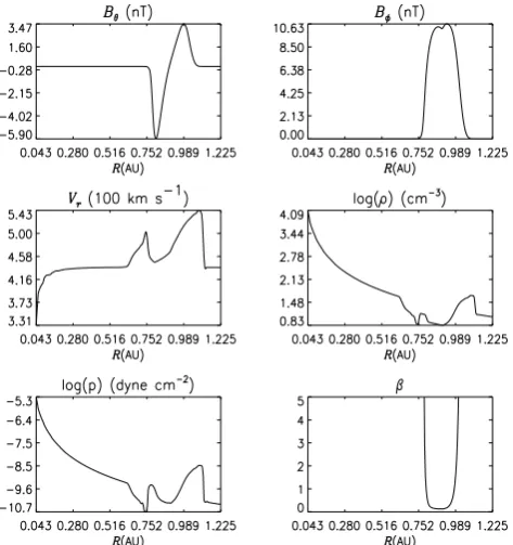
Fig. 2. Results from a 2.5-dimensional MHD simulation where the initial ICME velocity is double that of the solar wind. The six plots are cuts through the ICME alongθ = 0, and the panels show Bθ, Bφ, Vr, the density, pressure and plasma beta 2.57 days after the
initiation.
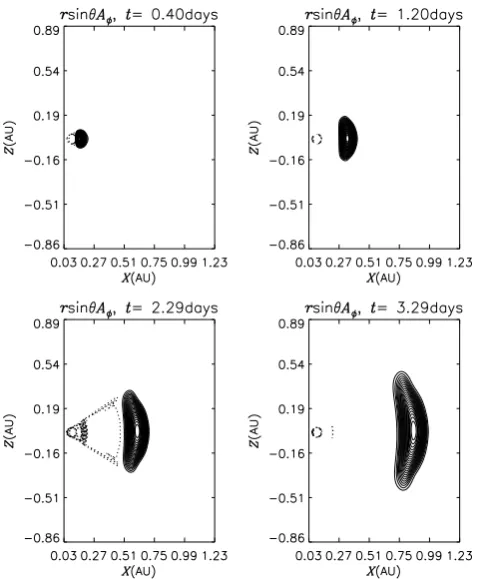
[image:6.595.47.284.62.314.2]Fig. 3. The magnetic field lines of the ICME projected onto the r−θplane for a case where the initial ICME moves at twice the solar wind speed. The four panels show the magnetic field at four different times in the outward journey.
Fig. 4. The plasma properties of the ICME projected onto ther−θ plane for a case where the initial ICME moves at twice the solar wind speed. The four panels show the change in Vrrelative to the
initial velocity, the angular velocity (Vθ), the change in the den-sity with respect to the initial value, and the magnitude of Bφ, 2.57 days after the initiation. Solid (dashed) lines indicate positive (neg-ative) contours. The maximum (minimum) contour values are 106 (31) km/s, 31 (−31) km/s, 120% (−80%) and 10.63 (0) nT, respec-tively.
is associated with a magnetic pressure that will tend to make the ICME expand.
Figure 2 shows a cut through the simulation along the θ = 0◦axis when the ICME is close to 1 AU, with the six panels showingBθ, Bφ, Vr, the density, pressure and plasma
beta. These plots can be contrasted directly with Fig. 1a. Fig-ure 3 shows the magnetic field lines projected into ther−θ plane for the fast ICME simulation at four different times and Fig. 4 shows contour plots of the change in the radial veloc-ity, the angular velocveloc-ity, the change in the density and the magnitude ofBφwhen the ICME is at 1 AU. Solid (dashed)
lines indicate positive (negative) contours.
It is apparent from Figs. 1 and 2 that the hydrodynamic and MHD simulations show qualitatively similar plasma structur-ing when a slice is taken through the symmetry axis of the simulation. A shock front preceeds the ICME in both cases. The trailing rarefaction wave has eaten its way into the ICME and in each case, the ICME rear can be defined by the lead-ing edge of the rear velocity enhancement at approximately 0.73 (0.8) AU in the MHD (hydrodynamic) model.
[image:6.595.46.282.420.685.2]Fig. 5. As Fig. 2, except that the initial ICME speed is now 0.5 times that of the solar wind. The results are shown 3.29 days after onset.
[image:7.595.49.285.63.327.2]Fig. 6. As Fig. 3, except that the initial ICME speed is now 0.5 times that of the solar wind. The results are shown 3.29 days after onset.
Fig. 7. As Fig. 4, except that the initial ICME speed is now 0.5 times that of the solar wind. The results are shown 3.29 days after onset. The maximum (minimum) contour values are 23 (−41) km/s, 17 (−17) km/s, 30% (−80%) and 9.88 (0) nT, respectively.
there is a region of compressed plasma corresponding to the initial region of enhanced magnetic field. This is due to the strong compression at the leading edge of the ICME as it ploughs into the initial solar wind. However, while the mag-netic field strength remains high throughout the ICME, the plasma density and pressure fall rapidly due to the effect of the trailing rarefaction wave, leading to a very cool, tenu-ous plasma that persists to the trailing edge of the ICME. As in the hydrodynamic case, the maximum velocity associated with the ICME relative to the solar wind has been decreased by the interaction with the background medium. Note though that the details of the plasma structure inside the ICME are qualitatively similar to that shown in Fig. 1, with small quan-titative differences which must be due to the impact that the magnetic field (through the magnetosonic wave speed) has on the propagation of the forward rarefaction wave.
[image:7.595.45.284.410.700.2]886 P. J. Cargill and J. M. Schmidt: Modelling interplanetary CMEs
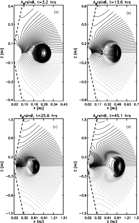
Fig. 8. The evolution of a magnetic flux rope in a radial solar wind magnetic field at four different times. Magnetic field lines projected onto ther−θplane are shown, with outwardly-directed solar wind field lines being shown as solid (dashed) lines above (below)θ=0. The ICME field has an anti-clockwise sense of rotation.
associated with the rarefaction-induced flow at the rear of the flux rope. This pushes the field lines forward, and the flux rope responds by expanding azimuthally. This effect was also noted in Cartesian geometry by Cargill et al. (1995; 1996). Unlike the hydrodynamic models, these MHD results also show the presence of a tangential discontinuity at the boundary between the ICME and solar wind plasma. It is clear from Figs. 2 and 5 that the ICME boundary is distinct from the shock waves, indicating the presence of a sheath of compressed solar wind plasma surrounding the ICME.
The plots of the plasma quantities show the large extent of the forward shock, extending through over 180◦ from the ICME. The shock also clearly extends well beyond the flux rope. For example, a spacecraft flying just above the magnetic structure would see rather a strong shock, but no magnetic cloud-like signature. This indicates that although the ICME, as defined by the magnetic field, influences a large region of space, the whole ICME including the shock
Fig. 9. As Fig. 9, except the ICME now encounters a current sheet atθ =0. Above (below)θ =0, field lines are directed away from (towards) the Sun. The ICME field has an anti-clockwise sense of rotation.
influences an even larger area.
We now contrast this with the case of a slow ICME. Fig-ure 5 shows a summary of the results along the θ = 0◦ line for the slow case. Note first that the ICME has taken 30% longer to reach 1 AU, a consequence of its slower initial speed. However, if we were to make a prediction of the ar-rival time based solely on the initial ICME speed, we would expect a factor 4 difference. This is compelling evidence for the importance of the interaction of the ICME with the solar wind in determining its arrival time and properties at 1 AU.
[image:8.595.46.279.63.437.2]able to propagate faster, thereby eliminating the rarefaction wave. The enhanced speed of propagation can be attributed to the enhanced magnetosonic speed inside the ICME when the magnetic field is present.
Figure 6 shows that the magnetic structure of the ICME also differs from the fast case. The ICME is more elongated in theθ direction, but narrower in the radial direction. We attribute this to the different way a deformable body responds to moving relative to a flow. When the ICME is accelerated into a flow, the flow slides around the side, but a flow at the rear does not flow around, thus, pushing the ICME edges outwards. Figure 7 confirms the absence of a leading shock, and the presence of a trailing shock, which is very flat when compared with the leading shock in Fig. 4.
3.2.2 Survival of flux rope structures to large distances Observations of magnetic flux ropes both at 1 AU and in the distant heliosphere by the Ulysses and Voyager spacecraft suggest that the flux rope structure of magnetic clouds is very stable when interacting with solar wind streams, shocks and other discontinuities. The fundamental reason for this stabil-ity is the strength of the magnetic tension force associated with the flux rope magnetic field. Thus, as the flux rope is squashed from various directions, the tension force resists any effort to distort it. We demonstrated this in our earlier Cartesian simulations of the interaction of a flux rope with an ambient plasma (Cargill et al., 1995; 1996). Although signif-icant fluid motions were generated in the external plasma by the motion of the flux rope, they only distorted the flux rope as opposed to shredding it. The same result is seen in Figs. 3 and 6. This point was emphasized by carrying out simula-tions of a flux tube (i.e. an ICME with straight magnetic field line, hence, lacking tension forces). Such a flux tube was gradually distorted until it eventually fell apart (Cargill et al., 1996).
One might then conclude that any structure that was a flux rope at the Sun would persist in this form to large radial dis-tances. However, recent results described by Cargill et al. (2000) suggest that this may not be the case. We showed that:
Bθ2 Bφ2
= B
2
θ0
Bφ20
r0
r
3ρ0
ρ , (6)
where a zero subscript denotes quantities evaluated at the start of the simulation (i.e. close to the Sun). This indi-cates that an ICME whose density fell as 1/r2would end up with a magnetic field predominantly along the flux rope axis (φdirection), effectively making it a flux tube, thus, suscepti-ble to shredding. By carrying out simulations of overexpand-ing ICMEs, Cargill et al. (2000) noted the preservation of a flux rope structure to 5 AU, and attributed this to the overex-pansion with an internal density falling off faster than 1/r3. This effect appears to only be of importance once over- ex-pansion sets in at large distances, and so it does not affect the ICME properties at 1 AU.
3.2.3 Magnetic reconnection between solar wind and ICME magnetic fields
ICMEs and the solar wind represent different magnetic flux systems, and, if conditions are right, can undergo magnetic reconnection with each other. Reconnection can lead to the peeling of magnetic field lines away from an ICME, and, hence, result in a loss of integrity, and perhaps ultimate as-similation into the solar wind magnetic field. Despite its presence in published work (Vandas et al., 1995), magnetic reconnection between ICMEs and the solar wind has been little studied.
It is easy to understand why reconnection could be of im-portance if we consider the motion of a flux rope in a unidi-rectional field (the case of ICME motion in a current sheet is distinct, and is discussed below). By definition, a magnetic flux rope has field lines pointing sunward and anti-sunward at opposite edges. If the solar wind field is unidirectional, then reconnection can happen at one (and only one) side of the flux rope. Cargill et al. (1996) performed Cartesian simula-tions of the motion of a magnetic flux rope in a unidirectional magnetic field. They showed that reconnection did indeed occur at a rate that was determined by the flows induced out-side the flux rope by its relative motion. However, the time scale for reconnection was quite long, so that the flux rope survived.
The more complicated case concerns the motion of mag-netic clouds in the vicinity of current sheets. Crooker et al. (1998) used a sample of 14 magnetic clouds from the ISEE-3 data set to argue that there is a close link between the ICME structure and the presence of interplanetary sector structure. This is currently an active research topic, and has not as of yet been addressed in numerical models using a magnetic cloud geometry.
We have carried out some MHD simulations on this topic. The results are shown in Figs. 8 and 9. The simulation model is the same as earlier, except that the initial magnetic field geometry consisted of a flux rope embedded in a distorted magnetic field, and the MHD equations are now solved over 180◦latitude. The full mathematical solution is discussed by Schmidt (2000), and these simulations will be presented in more detail elsewhere (Schmidt and Cargill, 2002). The cen-ter of the flux rope is located at 0.2 AU, and it has an initial diameter of 0.12 AU. There is a thermal over-pressure inside the flux rope by a factor of 3, so that some overexpansion will occur. In both cases, the initial ICME speed is twice that of the solar wind, as in Sect. 3.2.1.
888 P. J. Cargill and J. M. Schmidt: Modelling interplanetary CMEs are present only forθ >0, and in Fig. 9, they are present on
both sides of the ICME.
Figure 8 shows the magnetic field lines projected onto the r−θ plane at four different times. The field line notation is such that aboveθ = 0, outward field lines are solid, and belowθ =0, outward field lines are dashed. The same field lines are shown in each panel. This notation is used to em-phasis the topology change in the field (see Cargill et al., 1996). It is clear from the figure that magnetic reconnec-tion occurs at the upper leading edge of the flux rope. Here, oppositely directed field lines are pressed together, leading to a strongly driven situation where reconnection will be en-hanced. (It needs to be stated that our MHD code has no “artificial” diffusion: thus, any reconnection is due to the nu-merical diffusion due to truncation errors in the finite differ-ence scheme. We believe (see Cargill et al., 1996) that this is the optimal way to model reconnection computationally when the reconnection is strongly driven by external bound-ary conditions.) There is also some reconnection occurring at the trailing edge, where flows behind the ICME drive field lines together (Cargill et al., 1996).
At 1 AU, the ICME retains its integrity, but even so, roughly 10% of its original flux has been reconnected. This would be seen in spacecraft data as a region where the fa-miliar bidirectional electron heat flux reverts to a standard solar wind heat flux (Gosling, 1990). The reconnection rate also slows down as the ICME moves outward, and loses its outward velocity (the earlier arrival time than in Figs. 2–4 is partly due to the ICME beginning at a larger radial distance). Note also the lack of lateral expansion of the ICME, unlike that seen in Figs. 3 and 6. We attribute this to the magnetic tension force associated with the external field inhibiting any expansion.
In Fig. 9, the interplanetary field is now outward above the ICME, and inward below it, so that a current sheet is present atθ=0. Now reconnection occurs on both sides of the lead-ing edge of the ICME. The ICME size is now considerably less that the case with a radial field, as field line stripping now occurs on both sides. When the sense of field rotation inside the ICME is opposite to that presented here (i.e. paral-lel fields on both sides), the ICME can travel to 1 AU while maintaining its original magnetic structure. In this case, the reconnected field lines ahead of the flux rope now have no at-tachment to the Sun, and so they would appear as a drop-out in the heat flux (e.g. McComas et al., 1994).
4 Conclusions
Computational MHD models represent the best way to un-derstand the dynamics of ICMEs as they move through the solar wind. Through the simulations presented here, it is ap-parent that such simulations reveal physics that is not present in simpler analytical models (such as ICME interaction with, and distortion by, the solar wind). By choice of various pa-rameters, one can investigate different scenarios in a
con-trolled environment, and, hence, determine the important physical effects.
However, when one considers space weather forecasting, a very different conclusion as to the usefulness of MHD mod-els is reached. It is clear that the level of intensity of a geo-magnetic storm is largely determined by the IMF properties at 1 AU, especially on how long the field points southward, and on the minimum value of this component. Thus, an accu-rate forecasting of the IMF strength in an ICME is required in any realistic space weather forecasting tool. Both simula-tions and models have demonstrated that the IMF at 1 AU in an ICME is determined by the initial field properties in the solar corona, and perhaps on the cause of the initial CME ejection (Chen, 1996). However, it is well known that mea-surement of the coronal field strength is rendered difficult by the fact that the Zeeman effect is generally undetectable due to thermal line broadening there, although recent work has suggested possibilities of measuring the field using IR lines (Lin et al., 2000). Thus, the key parameter needed for useful forecasting is not readily available at this time.
Instead, we believe that forecasting must rely on (a) the proper analysis of all available observations, (b) the use of such analysis in establishing correlations between properties at the Sun and 1 AU, and in constructing statistical models whereby ICME properties at 1 AU can be forecast from solar conditions (see Gopalswamy et al., 2000; Owens and Cargill, 2002). The role of MHD modelling is then to determine the underlying physical principles governing these prediction models, and to guide forecasters into establishing further cor-relations that can improve their predictions.
Acknowledgements. J. S. acknowledges funding from the UK Par-ticle Physics and Astronomy Research Council. P. C. acknowledges financial support from ESA through the ALCATEL space weather team. P. C. is also grateful to Dan Spicer and Steve Zalesak for their advice and assistance in the computational aspects of this work, to Matt Owens for discussions on CME forecasting, and to all mem-bers of the ALCATEL space weather team for many stimulating discussions on the subject of space weather.
Topical Editor E. Antonucci thanks J. A. Klimchuk and another referee for their help in evaluating this paper.
References
Antiochos, S. K., DeVore, C. R., and Klimchuk, J. A.: A model for coronal mass ejections, Astrophys. J., 510, 485, 2000.
Brackbill, J. U. and Barnes, D. C.: The effect of non-zero∇·Bon the numerical solutions of the magnetohydrodynamic equations, J. Comput. Phys., 35, 426, 1980.
Burlaga, L. F.: Magnetic clouds: constant alpha force-free configu-rations, J. Geophys. Res., 93, 7217, 1988.
Burlaga, L. F. and Behannon, K. H.: Magnetic clouds: Voyager observations between 2 and 4 AU, Solar Phys., 81, 181, 1982. Burlaga, L. F., Sittler, E., Mariani, F. and Schwenn, R.: Magnetic
loop behind and interplanetary shock: Voyager, Helios and IMP8 observations, J. Geophys. Res., 86, 6673, 1981.
Cargill, P. J., Chen, J., Spicer, D. S., and Zalesak, S. T.: Geometry of interplanetary magnetic clouds, Geophys. Res. Lett., 22, 647, 1995.
Cargill, P. J., Chen, J., Spicer, D. S. and Zalesak, S. T.: MHD sim-ulations of the motion of magnetic flux tubes through a magne-tized plasma, J. Geophys. Res., 101, 4855, 1996.
Cargill, P. J., Schmidt, J., Spicer, D. S., and Zalesak, S. T.: The magnetic structure of over-expanding CMEs, J. Geophys. Res., 105, 7509, 2000.
Chen, J.: Theory of prominence eruption and propagation: inter-planetary consequences, J. Geophys. Res., 101, 27 499, 1996. Chen, J.: Physics of coronal mass ejections: a new paradigm for
solar eruptions, Space Sci Revs., 95, 165, 2001.
Chen, J. and Garren, D. A.: Interplanetary magnetic clouds: Topol-ogy and driving mechanism, Geophys. Res. Lett., 20, 2319, 1993.
Chen, J., Cargill, P. J., and Palmadesso, P. J.: Predicting geoeffec-tive solar wind structures, J. Geophys. Res., 102, 14 701, 1997. Crooker, N. U., Gosling, J. T., and Kahler, S. W.: Magnetic clouds
at sector boundaries, J. Geophys. Res., 103, 301, 1998.
Detman, T., Dryer, M., Yeh, T., Han, S. M., and Wu, S. T.: A time-dependent, three-dimensional MHD numerical study of inter-planetary magnetic draping around plasmoids in the solar wind, J. Geophys. Res., 96, 9531, 1991.
DeVore, C. R.: Flux-corrected transport techniques for multidimen-sional compressible MHD, J. Comp. Phys., 92, 142, 1991. Evans, C. R. and Hawley, J. F.: Simulation of
magnetohydrody-namic flows – A constrained transport method, Astrophys. J., 332, 659, 1988.
Forsyth, R. J., Balogh, A., Horbury, T. S., Erdos, G., Smith, E. J., and Burton, M. E. The heliospheric magnetic field at solar min-imum: Ulysses observations from pole to pole, Astron. Astro-phys., 316, 287, 1996.
Gopalswamy, N., Lara, A., Lepping, R. P., Kaiser, M. L., Berdichevsky, D., and St. Cyr, O. C.: Interplanetary acceleration of coronal mass ejections, Geophys. Res. Lett., 27, 145, 2000. Gosling, J. T.: Coronal mass ejections and magnetic flux ropes in
interplanetary space, in C. T. Russell et al., (Eds), Physics of magnetic flux ropes, AGU Monograph 58, AGU (Washington D. C.), 343, 1990.
Gosling, J. T., Bame, S. J., McComas, D. J., et al.: A forward-reverse shock pair in the solar wind driven by over- expansion of a CME: Ulysses observations, Geophys. Res. Lett., 21, 237, 1994.
Gosling, J. T., McComas, D. J., Phillips, J. L., et al.: A CME-driven solar wind disturbance observed at both low and high he-liographic latitudes, Geophys. Res. Lett., 22, 1753, 1995. Gosling, J. T. and Riley, P., The acceleration of slow coronal mass
ejections in the high-speed solar wind, Geophys. Res. Lett., 23, 2867, 1996.
Gosling, J. T., Riley, P., McComas, D. J., and Pizzo, V. J.: Overex-panding coronal mass ejections at high heliographic latitudes-Observations and simulations, J. Geophys. Res., 103, 1941, 1998.
Hammond, C. M., Crawford, G. K., Gosling, J. T., et al.: Latitudinal structure of a CME inferred from Ulysses and Geotail observa-tions, Geophys. Res. Lett., 22, 1169, 1995.
Hundhausen, A. J.: Coronal mass ejections, in: The many faces of the Sun, (Eds) Strong, K. T. et al., Springer, 143, 1999.
Hundhausen, A. J. and Gentry: The Propagation of Blast Waves in the Solar Wind, Astrophys. J. Supp, 73, 63, 1968.
Klein, L. W. and Burlaga, L. F.: Interplanetary magnetic clouds at
1 AU, J. Geophys. Res., 67, 613, 1982.
Klimchuk, J. A.: Theory of coronal mass ejections, in: Space Weather, (Eds) Song, P. et al., Geophysical Monograph, 125, (AGU, Washington DC), 143, 2001.
Kumar, P. and Rust, D. M.: Interplanetary magnetic clouds, helicity conservation, and current-core flux-ropes, J. Geophys. Res., 101, 15 667, 1996.
Lepping, R. P., Jones, J. A., and Burlaga, L. F.: Magnetic field struc-ture of interplanetary magnetic clouds at 1 AU, J. Geophys. Res., 95, 11 957, 1990.
Lin, H., Penn, M. J., and Tomczyk, S.: A new precise measurement of the coronal magnetic field strength, Astrophys. J. Lett., 541, L83, 2000.
Lindsay, G. M., Luhmann, J. G., Russell, C. T., and Gosling, J. T.: Relationships between CME speeds from coronagraph images and interplanetary characteristics of associated ICMEs, J. Geo-phys. Res., 104, 12 515, 1999.
Low, B. C.: Solar activity and the corona, Solar Phys., 167, 217, 1996.
Low, B. C.: Corona mass ejections, magnetic flux ropes, and solar magnetism, J. Geophys. Res., 106, 25 141, 2001.
McComas, D. J., Gosling, J. T., Hammond, C. M., Moldwin, M. B., Phillips, J. L., and Forsyth, R. J.: Magnetic reconnection ahead of a coronal mass ejection, Geophys. Res. Lett., 21, 1751, 1994. Mulligan, T. and Russell, C. T.: Multispacecraft modeling of the flux rope structure of interplanetary coronal mass ejec-tions: Cylindrically symmetric versus nonsymmetric topologies, J. Geophys. Res., 106, 10 581, 2001.
Mulligan, T., Russell, C. T., Anderson, B. J., and Acuna, M. H.: Multiple spacecraft flux rope modelling of the Bastille Day mag-netic cloud, Geophys. Res. Lett., 28, 4417, 2001.
Mulligan, T., Russell, C. T., and Luhmann, J. G.: Solar cycle evolu-tion of the structure of magnetic clouds in the inner heliosphere, Geophys. Res. Lett., 25, 2959, 1998.
Mulligan, T., Russell, C. T., Anderson, B. J., et al.: Intercomparison of NEAR and Wind interplanetary coronal mass ejection obser-vations, J. Geophys. Res., 104, 28 217, 1999.
Odstrcil, D. and Pizzo, V. J.: Distortion of the interplanetary mag-netic field by three-dimensional propagation of coronal mass ejections in a structured solar wind, J. Geophys. Res., 104, 483, 1999a.
Odstrcil, D. and Pizzo, V. J.: Three-dimensional propagation of coronal mass ejections in a structured solar wind flow 2. CME launched adjacent to the streamer belt, J. Geophys. Res., 104, 493, 1999b.
Owens, M. and Cargill, P. J.: Correlation of magnetic field intensi-ties and solar wind speeds for events observed by ACE, J. Geo-phys. Res., in press, 2002.
Reames, D. V.: Particle acceleration at the Sun and in the helio-sphere, Space Sci. Revs., 90, 413, 1999.
Riley, P., Gosling, J. T., and Pizzo, V. J.: A two-dimensional simu-lation of the radial and latitudinal evolution of a solar wind dis-turbance driven by a fast, high- pressure coronal mass ejection, J. Geophys. Res., 102, 14 677, 1997.
Schmidt, J. M.: Flux ropes embedded in a radial magnetic field: analytic solutions for the external magnetic field, Solar Phys., 197, 135, 2000.
Schmidt, J. M. and Cargill, P. J.: The evolution of magnetic flux ropes in sheared plasma flows, J. Plasma Phys., 64, 41, 2000. Schmidt, J. M. and Cargill, P. J.: Magnetic cloud evolution in a
890 P. J. Cargill and J. M. Schmidt: Modelling interplanetary CMEs CME and the solar wind magnetic field, J. Geophys. Res.,
sub-mitted, 2002.
Spicer, D. S.: private communication with P. Cargill, 1993. Tsurutani, B. T., Smith, E. J., Gonzalez, W. D., Tang, F., and
Aka-sofu, S. I.: Origin of interplanetary southward magnetic fields re-sponsible for major magnetic storms near solar maximum (1978– 1979), J. Geophys. Res., 93, 8519, 1998.
Vandas, M., Fischer, S., Pelant, P., and Geranios, A.: Spheroidal models of magnetic clouds and comparison with spacecraft mea-surements, J. Geophys. Res., 98, 11 467, 1993.
Vandas, M., Fischer, S., Dryer, M., Smith, Z., and Detman, T.: Sim-ulation of magnetic cloud propagation in the inner heliosphere
in two-dimensions: 1. loop perpendicular to the ecliptic plane, J. Geophys. Res., 100, 12 285, 1995.
Vrsnak, B.: Deceleration of coronal mass ejections, Solar Phys., 202, 173, 2001.
Wu, S. T., Guo, W. P., Michels., D. J, and Burlaga, L. F.: MHD description of the dynamical relationships between a flux rope, streamer, coronal mass ejection, and magnetic cloud: analysis of the January 1997 Sun-Earth connection event, J. Geophys. Res., 104, 14 789, 1999.