linear_regression_ch3.pdf

(1)

Linear regression

• Linear regression is a simple approach to supervised learning. It assumes that the dependence of Y on

X1, X2, . . . Xp is linear.

• True regression functions are never linear!

SLDM III cHastie & Tibshirani - March 7, 2013 Linear Regression 71

Linearity assumption?

η(x) =β0+β1x1+β2x2+. . . βpxp

Almost always thought of as an approximation to the truth. Functions in nature are rarely linear.

2 4 6 8

3

4

5

6

7

X

f(X)

(2)

Linear regression

η(x) =β0+β1x1+β2x2+. . . βpxp

2 4 6 8

3

4

5

6

7

X

f(X)

(3)

Linear regression

η(x) =β0+β1x1+β2x2+. . . βpxp

2 4 6 8

3

4

5

6

7

X

f(X)

(4)

Linear regression for the advertising data

Consider the advertising data shown on the next slide.

Questions we might ask:

• Is there a relationship between advertising budget and sales?

• How strong is the relationship between advertising budget and sales?

• Which media contribute to sales?

• How accurately can we predict future sales?

• Is the relationship linear?

(5)

Advertising data

0 50 100 200 300

5 10 15 20 25 TV Sales

0 10 20 30 40 50

5 10 15 20 25 Radio Sales

0 20 40 60 80 100

(6)

Simple linear regression using a single predictor

X

.

• We assume a model

Y =β0+β1X+,

where β0 and β1 are two unknown constants that represent

theintercept and slope, also known as coefficientsor

parameters, and is the error term.

• Given some estimates ˆβ0 and ˆβ1 for the model coefficients,

we predict future sales using

ˆ

y= ˆβ0+ ˆβ1x,

(7)

Estimation of the parameters by least squares

• Let ˆyi= ˆβ0+ ˆβ1xi be the prediction for Y based on the ith

value of X. Then ei =yi−yˆi represents theith residual

• We define the residual sum of squares (RSS) as RSS =e2₁+e2₂+_{· · ·}+e2_n,

or equivalently as

RSS = (y1−β0ˆ −β1x1ˆ )2+(y2−β0ˆ −β1x2ˆ )2+. . .+(yn−β0ˆ −β1xˆ n)2.

• The least squares approach chooses ˆβ0 and ˆβ1 to minimize

the RSS. The minimizing values can be shown to be

ˆ

β1 =

Pn

i=1(xi−x¯)(yi−y¯)

Pn

i=1(xi−x¯)2

,

ˆ

β0 = ¯y−βˆ1x,¯

where ¯y_≡ _n1Pn_i₌₁yi and ¯x≡ 1_n

Pn

i=1xi are the sample

(8)

Estimation of the parameters by least squares

or equivalently as

ˆ

β1 =

Pn

i=1(xi−x¯)2

,

ˆ

β0 = ¯y−βˆ1x,¯

where ¯y_≡ _n1Pn_i₌₁yi and ¯x≡ 1_n

Pn

i=1xi are the sample

(9)

Estimation of the parameters by least squares

or equivalently as

ˆ

β1 =

Pn

i=1(xi−x¯)2

,

ˆ

β0 = ¯y−βˆ1x,¯

where ¯y_≡ 1_nPn_i₌₁yi and ¯x≡ 1_nPni=1xi are the sample

(10)

Example: advertising data

4 3. Linear Regression

between theith observed response value and theith response value that is predicted by our linear model. We define theresidual sum of squares(RSS)

residual sum of squares

as

RSS =e2

1+e22+· · ·+e2n,

or equivalently as

RSS = (y1−_β0ˆ₋_β1x1ˆ ₎2_{+ (}_y2₋_β0ˆ₋_β1x2ˆ ₎2₊_{. . .}_{+ (}_y

n−β0ˆ−β1xˆ n)2.(3.3)

The least squares approach chooses ˆβ0and ˆβ1to minimize the RSS. Using some calculus, one can show that the minimizers are

ˆ β1=

Pn

i=1(xi−x¯)(yi−¯y) Pn

i=1(xi−x¯)2

,

ˆ

β0= ¯y−β1ˆx,¯

(3.4)

where ¯y≡1

n Pn

i=1yiand ¯x≡1n Pn

i=1xiare the sample means. In other

words, (3.4) defines theleast squares coefficient estimatesfor simple linear regression.

0 50 100 150 200 250 300

5 10 15 20 25 TV Sales

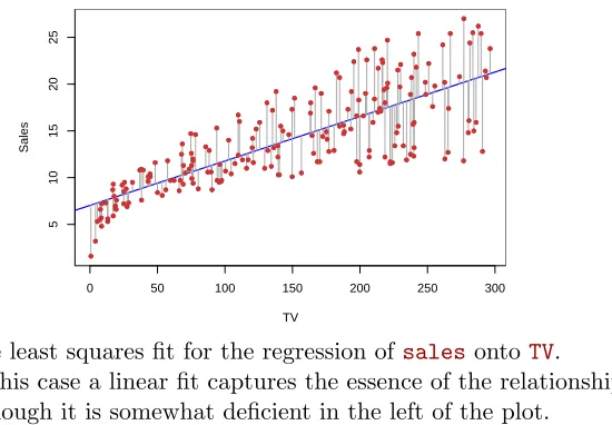
FIGURE 3.1.For theAdvertisingdata, the least squares fit for the regression

ofsalesontoTVis shown. The fit is found by minimizing the sum of squared

errors. Each grey line segment represents an error, and the fit makes a compro-mise by averaging their squares. In this case a linear fit captures the essence of the relationship, although it is somewhat deficient in the left of the plot.

Figure 3.1 displays the simple linear regression fit to theAdvertising

data, where ˆβ0= 7.03 and ˆβ1= 0.0475. In other words, according to this

The least squares fit for the regression ofsalesonto TV.

(11)

Assessing the Accuracy of the Coefficient Estimates

• The standard error of an estimator reflects how it varies under repeated sampling. We have

SE( ˆβ1) 2

= σ

2

Pn

i=1(xi−x¯)2

, SE( ˆβ0) 2

=σ2

1 n + ¯ x2 Pn

i=1(xi−x¯)2

,

where σ2= Var()

• These standard errors can be used to compute confidence intervals. A 95% confidence interval is defined as a range of values such that with 95% probability, the range will contain the true unknown value of the parameter. It has the form

ˆ

(12)

Assessing the Accuracy of the Coefficient Estimates

• The standard error of an estimator reflects how it varies under repeated sampling. We have

SE( ˆβ1) 2

= σ

2

Pn

i=1(xi−x¯)2

, SE( ˆβ0) 2

=σ2

1 n + ¯ x2 Pn

i=1(xi−x¯)2

,

where σ2= Var()

• These standard errors can be used to compute confidence intervals. A 95% confidence interval is defined as a range of values such that with 95% probability, the range will contain the true unknown value of the parameter. It has the form

ˆ

(13)

Confidence intervals — continued

That is, there is approximately a 95% chance that the interval

h

ˆ

β1−2·SE( ˆβ1), β1ˆ + 2·SE( ˆβ1)i

will contain the true value ofβ1 (under a scenario where we got

repeated samples like the present sample)

For the advertising data, the 95% confidence interval forβ1 is

(14)

Confidence intervals — continued

That is, there is approximately a 95% chance that the interval

h

ˆ

β1−2·SE( ˆβ1), β1ˆ + 2·SE( ˆβ1)i

will contain the true value ofβ1 (under a scenario where we got

repeated samples like the present sample)

For the advertising data, the 95% confidence interval forβ1 is

(15)

Hypothesis testing

• Standard errors can also be used to perform hypothesis testson the coefficients. The most common hypothesis test involves testing the null hypothesisof

H0 : There is no relationship between X andY

versus the alternative hypothesis

HA: There is some relationship between X and Y .

• Mathematically, this corresponds to testing

H0:β1= 0

versus

HA:β1 6= 0,

since ifβ1= 0 then the model reduces to Y =β0+, and

(16)

Hypothesis testing

• Standard errors can also be used to perform hypothesis testson the coefficients. The most common hypothesis test involves testing the null hypothesisof

H0 : There is no relationship between X andY

versus the alternative hypothesis

HA: There is some relationship between X and Y .

• Mathematically, this corresponds to testing

H0:β1= 0

versus

HA:β1 6= 0,

since ifβ1= 0 then the model reduces to Y =β0+, and

(17)

Hypothesis testing — continued

• To test the null hypothesis, we compute a t-statistic, given by

t= β1ˆ −0 SE( ˆβ1) ,

• This will have a t-distribution with n₋2 degrees of freedom, assuming β1 = 0.

• Using statistical software, it is easy to compute the

(18)

Results for the advertising data

Coefficient Std. Error t-statistic p-value

Intercept 7.0325 0.4578 15.36 <0.0001

(19)

Assessing the Overall Accuracy of the Model

• We compute the Residual Standard Error

RSE =

r

1

n−2RSS =

v u u

t 1

n−2

n

X

i=1

(yi−yˆi)2,

where theresidual sum-of-squaresis RSS=Pn_i₌₁(yi−yˆi)2.

• R-squared or fraction of variance explained is

R2= TSS−RSS TSS = 1−

RSS TSS

where TSS =Pn_i₌₁(yi−y¯)2 is the total sum of squares.

• It can be shown that in this simple linear regression setting that R2 =r2, wherer is the correlation betweenX and Y:

r =

Pn

i=1(xi−x)(yi−y)

pPn

i=1(xi−x)2pPni=1(yi−y)2

(20)

Assessing the Overall Accuracy of the Model

RSE =

r

1

n−2RSS =

v u u

t 1

n−2

n

X

i=1

(yi−yˆi)2,

R2 = TSS−RSS TSS = 1−

RSS TSS

r =

Pn

i=1(xi−x)(yi−y)

pPn

(21)

Assessing the Overall Accuracy of the Model

RSE =

r

1

n−2RSS =

v u u

t 1

n−2

n

X

i=1

(yi−yˆi)2,

R2 = TSS−RSS TSS = 1−

RSS TSS

r=

Pn

i=1(xi−x)(yi−y)

pPn

(22)

Advertising data results

Quantity Value

Residual Standard Error 3.26

R2 0.612

(23)

Multiple Linear Regression

• Here our model is

Y =β0+β1X1+β2X2+· · ·+βpXp+,

• We interpretβj as theaverageeffect on Y of a one unit

increase inXj,holding all other predictors fixed. In the

advertising example, the model becomes

(24)

Interpreting regression coefficients

• The ideal scenario is when the predictors are uncorrelated — a balanced design:

- Each coefficient can be estimated and tested separately. - Interpretations such as“a unit change inXj is associated

with aβj change inY, while all the other variables stay

fixed”, are possible.

• Correlations amongst predictors cause problems:

- The variance of all coefficients tends to increase, sometimes dramatically

- Interpretations become hazardous — whenXj changes, everything else changes.

(25)

The woes of (interpreting) regression coefficients

“Data Analysis and Regression” Mosteller and Tukey 1977

• a regression coefficient βj estimates the expected change in

Y per unit change inXj,with all other predictors held fixed. But predictors usually change together!

• Example: Y total amount of change in your pocket;

X1= # of coins; X2= # of pennies, nickels and dimes. By

itself, regression coefficient of Y on X2 will be>0. But how about withX1 in model?

• Y= number of tackles by a football player in a season; W

(26)

The woes of (interpreting) regression coefficients

itself, regression coefficient of Y onX2 will be>0. But how about withX1 in model?

(27)

The woes of (interpreting) regression coefficients

itself, regression coefficient of Y onX2 will be>0. But how about withX1 in model?

(28)

Two quotes by famous Statisticians

“Essentially, all models are wrong, but some are useful”

George Box

“The only way to find out what will happen when a complex system is disturbed is to disturb the system, not merely to observe it passively”

(29)

Two quotes by famous Statisticians

“Essentially, all models are wrong, but some are useful”

George Box

“The only way to find out what will happen when a complex system is disturbed is to disturb the system, not merely to observe it passively”

(30)

Estimation and Prediction for Multiple Regression

• Given estimates ˆβ0,βˆ1, . . .βˆp, we can make predictions

using the formula

ˆ

y= ˆβ0+ ˆβ1x1+ ˆβ2x2+· · ·+ ˆβpxp.

• We estimate β0, β1, . . . , βp as the values that minimize the

sum of squared residuals

RSS =

n

X

i=1

(yi−yˆi)2

=

n

X

i=1

(yi−βˆ0−βˆ1xi1−βˆ2xi2− · · · −βˆpxip)2.

This is done using standard statistical software. The values ˆ

β0,β1, . . . ,ˆ βˆp that minimize RSS are the multiple least

(31)

3.2 Multiple Linear Regression 15

X1

X2

Y

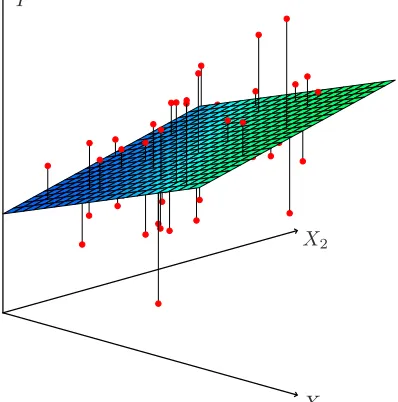
FIGURE 3.4.In a three-dimensional setting, with two predictors and one re-sponse, the least squares regression line becomes a plane. The plane is chosen to minimize the sum of the squared vertical distances between each observation (shown in red) and the plane.

The parameters are estimated using the same least squares approach that we saw in the context of simple linear regression. We chooseβ0, β1, . . . , βp

to minimize the sum of squared residuals

RSS =

n

X

i=1

(yi−yiˆ)2

=

n

X

i=1

(yi−βˆ0−βˆ1xi1−βˆ2xi2− · · · −βpxipˆ )2. (3.22)

The values ˆβ0,βˆ1, . . . ,βpˆ that minimize (3.22) are the multiple least squares

regression coefficient estimates. Unlike the simple linear regression esti-mates given in (3.4), the multiple regression coefficient estiesti-mates have somewhat complicated forms that are most easily represented using ma-trix algebra. For this reason, we do not provide them here. Any statistical software package can be used to compute these coefficient estimates, and

later in this chapter we will show how this can be done in R. Figure 3.4

illustrates an example of the least squares fit to a toy data set withp= 2

predictors.

Table 3.4 displays the multiple regression coefficient estimates when TV, radio, and newspaper advertising budgets are used to predict product sales

(32)

Results for advertising data

Intercept 2.939 0.3119 9.42 <0.0001

TV 0.046 0.0014 32.81 <0.0001

radio 0.189 0.0086 21.89 <0.0001

newspaper -0.001 0.0059 -0.18 0.8599

Correlations:

TV radio newspaper sales

TV 1.0000 0.0548 0.0567 0.7822

radio 1.0000 0.3541 0.5762

newspaper 1.0000 0.2283

(33)

Some important questions

1. Is at least one of the predictors X1, X2, . . . , Xp useful in predicting the response?

2. Do all the predictors help to explain Y, or is only a subset of the predictors useful?

3. How well does the model fit the data?

(34)

Some important questions

(35)

Some important questions

(36)

Some important questions

(37)

Is at least one predictor useful?

For the first question, we can use the F-statistic

F = (TSS−RSS)/p

RSS/(n₋p₋1) ∼Fp,n−p−1

Quantity Value

Residual Standard Error 1.69

R2 _0.897

(38)

Deciding on the important variables

• The most direct approach is called all subsetsorbest subsets regression: we compute the least squares fit for all possible subsets and then choose between them based on some criterion that balances training error with model size.

• However we often can’t examine all possible models, since they are 2p _{of them; for example when} _p_{= 40 there are}

over a billion models!

(39)

Deciding on the important variables

• The most direct approach is called all subsetsorbest subsets regression: we compute the least squares fit for all possible subsets and then choose between them based on some criterion that balances training error with model size.

• However we often can’t examine all possible models, since they are 2p _{of them; for example when} _p_{= 40 there are}

over a billion models!

(40)

Forward selection

• Begin with the null model— a model that contains an intercept but no predictors.

• Fitp simple linear regressions and add to the null model the variable that results in the lowest RSS.

• Add to that model the variable that results in the lowest RSS amongst all two-variable models.

(41)

Backward selection

• Start with all variables in the model.

• Remove the variable with the largest p-value — that is, the variable that is the least statistically significant.

• The new (p−1)-variable model is fit, and the variable with the largest p-value is removed.

(42)

Model selection — continued

• Later we discuss more systematic criteria for choosing an “optimal” member in the path of models produced by forward or backward stepwise selection.

• These include Mallow’s Cp,Akaike information criterion

(AIC),Bayesian information criterion (BIC),adjusted R2

(43)

Other Considerations in the Regression Model

Qualitative Predictors

• Some predictors are not quantitativebut arequalitative, taking a discrete set of values.

• These are also called categorical predictors orfactor variables.

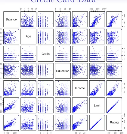
• See for example the scatterplot matrix of the credit card data in the next slide.

In addition to the 7 quantitative variables shown, there are four qualitative variables: gender,student(student status), status(marital status), andethnicity

(44)

Credit Card Data

Balance

20 4060 80100 5 10 15 20 2000 8000 14000

0 500 1500 20 40 60 80 100 Age Cards 2 4 6 8 5 10 15 20 Education Income 50 100 150 2000 8000 14000 Limit

0500 1500 2 4 6 8 50100150 200 600 1000

200

600

1000

Rating

FIGURE 3.6.TheCreditdata set contains information aboutbalance,age,

cards,education,income,limit, andratingfor a number of potential

cus-tomers.

and use this variable as a predictor in the regression equation. This results in the model

yi=β0+β1xi+ǫi= (

β0+β1+ǫi ifith person is female

β0+ǫi ifith person is male.

(3.27)

Nowβ0can be interpreted as the average credit card balance among males, β0+β1as the average credit card balance among females, andβ1as the average difference in credit card balance between females and males.

Table 3.7 displays the coefficient estimates and other information asso-ciated with the model (3.27). The average credit card debt for males is estimated to be $509.80, whereas females are estimated to carry $19.73 in additional debt for a total of $509.80 + $19.73 = $529.53. However, we notice that the p-value for the dummy variable is very high. This indicates

(45)

Qualitative Predictors — continued

Example: investigate differences in credit card balance between males and females, ignoring the other variables. We create a new variable

xi =

(

1 ifith person is female 0 ifith person is male

Resulting model:

yi =β0+β1xi+i=

(

β0+β1+i ifith person is female

β0+i ifith person is male.

(46)

Credit card data — continued

Results for gender model:

Intercept 509.80 33.13 15.389 <0.0001

(47)

Qualitative predictors with more than two levels

• With more than two levels, we create additional dummy variables. For example, for the ethnicityvariable we create two dummy variables. The first could be

xi1=

(

1 ifith person is Asian 0 ifith person is not Asian,

and the second could be

xi2 =

(

(48)

Qualitative predictors with more than two levels —

continued.

• Then both of these variables can be used in the regression equation, in order to obtain the model

yi=β0+β1xi1+β2xi2+i=   

 

β0+β1+i ifith person is Asian β0+β2+i ifith person is Caucasian

β0+i ifith person is AA.

• There will always be one fewer dummy variable than the number of levels. The level with no dummy variable — African American in this example — is known as the

(49)

Results for ethnicity

Intercept 531.00 46.32 11.464 <0.0001

ethnicity[Asian] -18.69 65.02 -0.287 0.7740

(50)

Extensions of the Linear Model

Removing the additive assumption: interactionsand

nonlinearity

Interactions:

• In our previous analysis of theAdvertisingdata, we

assumed that the effect onsales of increasing one

advertising medium is independent of the amount spent on the other media.

• For example, the linear model

\

sales=β0+β1×TV+β2×radio+β3×newspaper

states that the average effect on salesof a one-unit increase inTV is always β1, regardless of the amount spent

(51)

Interactions — continued

• But suppose that spending money on radio advertising actually increases the effectiveness of TV advertising, so that the slope term for TVshould increase asradio

increases.

• In this situation, given a fixed budget of $100,000,

spending half on radioand half on TV may increasesales

more than allocating the entire amount to eitherTV or to

radio.

(52)

Interaction in the Advertising data?

3.2 Multiple Linear Regression 81

Sales

Radio TV

FIGURE 3.5.For theAdvertisingdata, a linear regression fit tosalesusing

TVandradioas predictors. From the pattern of the residuals, we can see that there is a pronounced non-linear relationship in the data.

which simplifies to (3.15) for a simple linear regression. Thus, models with more variables can have higher RSE if the decrease in RSS is small relative to the increase inp.

In addition to looking at the RSE andR2_{statistics just discussed, it can} be useful to plot the data. Graphical summaries can reveal problems with a model that are not visible from numerical statistics. For example, Fig-ure 3.5 displays a three-dimensional plot ofTVandradioversussales. We see that some observations lie above and some observations lie below the least squares regression plane. Notice that there is a clear pattern of nega-tive residuals, followed by posinega-tive residuals, followed by neganega-tive residuals. In particular, the linear model seems to overestimatesalesfor instances in which most of the advertising money was spent exclusively on either

TVorradio. It underestimatessalesfor instances where the budget was split between the two media. This pronounced non-linear pattern cannot be modeled accurately using linear regression. It suggests asynergyor inter-actioneffect between the advertising media, whereby combining the media together results in a bigger boost to sales than using any single medium. In Section 3.3.2, we will discuss extending the linear model to accommodate such synergistic effects through the use of interaction terms.

When levels of eitherTV orradioare low, then the true sales

are lower than predicted by the linear model.

But when advertising is split between the two media, then the model tends to underestimatesales.

(53)

Modelling interactions — Advertising data

Model takes the form

sales = β0+β1×TV+β2×radio+β3×(radio×TV) +

= β0+ (β1+β3×radio)×TV+β2×radio+.

Results:

Intercept 6.7502 0.248 27.23 <0.0001

TV 0.0191 0.002 12.70 <0.0001

radio 0.0289 0.009 3.24 0.0014

(54)

Interpretation

• The results in this table suggests that interactions are important.

• The p-value for the interaction termTV_×radio is

extremely low, indicating that there is strong evidence for

HA:β3 6= 0.

• The R2 _{for the interaction model is 96}_._{8%, compared to}

only 89.7% for the model that predicts salesusing TVand

(55)

Interpretation — continued

• This means that (96.8₋89.7)/(100₋89.7) = 69% of the variability in sales that remains after fitting the additive

model has been explained by the interaction term.

• The coefficient estimates in the table suggest that an increase in TV advertising of $1,000 is associated with increased sales of

( ˆβ1+ ˆβ3×radio)×1000 = 19 + 1.1×radio units.

• An increase in radio advertising of $1,000 will be associated with an increase in sales of

(56)

Hierarchy

• Sometimes it is the case that an interaction term has a very small p-value, but the associated main effects (in this case,TV and radio) do not.

• The hierarchy principle:

(57)

Hierarchy — continued

• The rationale for this principle is that interactions are hard to interpret in a model without main effects — their meaning is changed.

(58)

Interactions between qualitative and quantitative

variables

Consider theCreditdata set, and suppose that we wish to predictbalance usingincome(quantitative) and student

(qualitative).

Without an interaction term, the model takes the form

balancei ≈ β0+β1×incomei+ (

β2 ifith person is a student 0 ifith person is not a student

= β1×incomei+ (

β0+β2 ifith person is a student

(59)

With interactions, it takes the form

β2+β3×incomei if student

0 if not student

=

(

(60)

0 50 100 150

200 600 1000 1400 Income Balance

0 50 100 150

200 600 1000 1400 Income Balance student non−student

FIGURE 3.7.For theCredit data, the least squares lines are shown for pre-diction ofbalancefromincomefor students and non-students.Left:The model (3.34) was fit. There is no interaction betweenincomeand student.Right:The model (3.35) was fit. There is an interaction term betweenincomeandstudent.

takes the form

β2 ifith person is a student

0 ifith person is not a student

= β1×incomei+ (

β0+β2 ifith person is a student

β0 ifith person is not a student.

(3.34)

Notice that this amounts to fitting two parallel lines to the data, one for students and one for non-students. The lines for students and non-students have different intercepts,β0+β2 versusβ0, but the same slope, β1. This

is illustrated in the left-hand panel of Figure 3.7. The fact that the lines are parallel means that the average effect onbalanceof a one-unit increase inincomedoes not depend on whether or not the individual is a student. This represents a potentially serious limitation of the model, since in fact a change inincomemay have a very different effect on the credit card balance of a student versus a non-student.

This limitation can be addressed by adding an interaction variable, cre-ated by multiplying income with the dummy variable for student. Our model now becomes

β2+β3×incomei if student

0 if not student

=

(

(β0+β2) + (β1+β3)×incomei if student

β0+β1×incomei if not student

(3.35)

Once again, we have two different regression lines for the students and the non-students. But now those regression lines have different intercepts,

Credit data; Left: no interaction betweenincomeand student. Right: with an interaction term betweenincomeand student.

(61)

Non-linear effects of predictors

polynomial regression onAutodata

3.3 Other Considerations in the Regression Model 91

50 100 150 200

10 20 30 40 50 Horsepower

Miles per gallon

Linear Degree 2 Degree 5

FIGURE 3.8.TheAutodata set. For a number of cars,mpgandhorsepowerare shown. The linear regression fit is shown in orange. The linear regression fit for a model that includeshorsepower2is shown as blue curve. The linear regression fit for a model that includes all polynomials of horsepower up to fifth-degree is shown in green.

β0+β2versusβ0, as well as different slopes,β1+β3versusβ1. This allows for

the possibility that changes in income may affect the credit card balances of students and non-students differently. The right-hand panel of Figure 3.7 shows the estimated relationships betweenincomeandbalancefor students and non-students in the model (3.35). We note that the slope for students is lower than the slope for non-students. This suggests that increases in income are associated with smaller increases in credit card balance among students as compared to non-students.

Non-Linear Relationships

As discussed previously, the linear regression model (3.19) assumes a linear relationship between the response and predictors. But in some cases, the true relationship between the response and the predictors may be non-linear. Here we present a very simple way to directly extend the linear model to accommodate non-linear relationships, using polynomial regression. In

polynomial regression later chapters, we will present more complex approaches for performing

non-linear fits in more general settings.

Consider Figure 3.8, in which the mpg(gas mileage in miles per gallon) versushorsepoweris shown for a number of cars in theAutodata set. The orange line represents the linear regression fit. There is a pronounced

(62)

The figure suggests that

mpg=β0+β1×horsepower+β2×horsepower2+

may provide a better fit.

Intercept 56.9001 1.8004 31.6 <0.0001

horsepower -0.4662 0.0311 -15.0 <0.0001

(63)