Effect of Wind Speed and Load Correlation on ELCC of Wind
Turbine Generator
M. A. Armin*, H. Rajabi Mashhadi**(C.A.)
Abstract: Utilization of wind turbines as economic and green production units, poses new challenges to the power system planners, mainly due to the stochastic nature of the wind, adding a new source of uncertainty to the power system. Different types of distribution and correlation between this random variable and the system load make conventional method inappropriate for modeling such a correlation. In this paper, the correlation between the wind speed and system load is modeled using Copula, a mathematical tool recently used in the field of the applied science. As the effect of the correlation coefficient is the main concern, the copula modeling technique allows simulating various scenarios with different correlations. The conducted simulations in this paper reveal that the wind speed correlation with the load has a significant effect on the system reliability indices, such as Expected Energy Not Served (EENS) and Loss Of Load Probability (LOLP). Moreover, in this paper the effect of the correlation coefficient on the Effective Load Carrying Capability (ELCC) of the wind turbines is analyzed, too. To perform the aforementioned simulations and analyses, the modified RBTS with an additional wind farm is used.
Keywords: Copula, Correlation, Effective Load Carrying Capability, Reliability Indices, Wind Power Generation.
1 Introduction1
1.1 Motivation
Penetration of wind energy into the power system has been increased during the recent years. The Rising cost of the fossil fuels and the negative environmental impacts of the conventional generations have provided strong incentives for wind power deployment. The developed countries replace the conventional units with the Wind Turbine Generators (WTGs), mainly due to their environmental policies and green energy plans. On the other hand, in the developing countries, where utilities face increasing demand over the planning period, WTGs are seen as an economical source of power and governments and experts consider these cost-effective energy sources in the generation expansion planning.
However, the wind speed is variable and uncontrollable. These phenomena cause the mean value
Iranian Journal of Electrical & Electronic Engineering, 2015. Paper first received 1 Dec. 2014 and in revised form 18 Jan. 2015. * The Author is with the Department of Electrical Engineering, Ferdowsi University of Mashhad, Mashhad, Iran.
** The Author is with the Department of Electrical Engineering and the Center of Excellence on Soft Computing and Intelligent Information Processing, Ferdowsi University of Mashhad, Mashhad, Iran.
E-mails: [email protected] and [email protected].
of the output power to be less than the turbine nameplate. In other words, the capacity factor for a WTG is much less than a similar conventional unit. The reserve capacities are the ancillary service to overcome these challenge [1]. In addition to the considerable uncertainty of the wind speed, the value of the correlation factor between the Wind Speed (WS) and the load affects the power system performance. Hence, considering power system planning aspects, the capacity and the location of the WTGs should be carefully chosen.
To determine the proper capacity of the wind generation, the Effective Load Carrying Capability (ELCC) of the WTGs is used. The index indicates the capability of the WTG to serve the load. For the calculation of the ELCC, models are required to represent the complicated behavior of the wind and load and their correlation.
1.2 Literature Review
The concept of the ELCC has been widely used in the context of the long term planning of the wind farm ([2, 3]). ELCC has been used as an index for the wind farms in [4] and effect of the wind farms location on the ELCC has been analyzed. Similar work has been carried out in [5]. In these researches, wind speed and load have been modeled by the sequential Monte Carlo. However,
the correlation between the wind speed and load has not been addressed since this issue has not been the main concern of the authors.
Early works regarding the correlation between the wind speed and load have been published in 1980s. The effects of the correlation between the load and wind have been indicated in [6] and [7]. In [7], the authors have addressed the dependency between the wind and load in an Irish case study. Load and wind correlation coefficient for this study was reported about 0.15 - 0.20, which was ignored to avoid the computational complexity. Seasonal correlation between the load and wind has been pointed out in [8]. In a study for the U.S. Department of Energy, it has been emphasized that these correlations “do exist” and have a complex pattern [9]. In [10], the authors claim a negative correlation between load and wind “in most systems.” Such dependency can affect system analysis and should be accurately represented. In [11], a method has been presented for modeling the correlation between the wind speed, solar insolation and load curves. This study has concluded that such a correlation, as an important factor, must be considered in the reliability evaluations.
Modeling these correlations faces two main challenges. First, these correlations change site by site and have different values in the different systems. So far, researchers have used historical data to include the impact of wind speed-load correlation (WLC) on the power system. A simple method is to consider the wind production as negative load and then add it to the real load data. This approach has been reported in several cases such as California in 2004 [12], Minnesota state [13] and New York [14] in 2006, Ireland [15], and India [16]. While this method is practical but can be used just for specified case studies. Any changes in load or wind pattern cannot be considered in this method.
The second challenge is associated with the different distributions of the wind and load. This causes the dependency between the wind and load to be nonlinear. Copula, which recently has been reported as a powerful tool for modeling [17], can be used to generate a joint probability function. This technique allows combining different distributions, derived from the historical data, based on a dependency level. Copula method is based on the Sklar theorem, presented in 1956. Copula has been used in the different fields of science, such as weather forecast, mechanics, and particularly in finance. In [17] and [18] copula has been used to model the correlation between the wind generations in the Netherlands. Similar works have been conducted for the Swiss grid [19] and Davarzan distribution system in Iran [20]. In all these works, an empirical copula approach based on the historical data has been employed to extract and model the cumulative distribution of the equivalent load.
1.3 Approach and Contributions
The main goal of this paper is to include the effect of
the WLC in the calculation of the ELCC of a WTG. In this paper, the ELCC is computed based on the reliability analysis. Two well-known reliability indices, including the Loss Of Load Probability (LOLP) and Expected Energy Not Served (EENS) are used for this purpose.
As wind and load distributions and their correlation have a direct effect on the power system reliability indices, it is necessary to consider the WLC in the ELCC computation. Correlation degree can be adjusted based on the statistical analysis of the historical data. In the proposed copula-based modeling, the correlation can be adjusted in order to cover other likely situations. The ELCC of a wind generator is calculated by Monte Carlo simulation for different values of the correlation coefficient between the load and wind. The obtained results show that the WLC plays a key role in the value of the ELCC corresponding to a WTG. Based on the simulation results, the capacity factor of a WTG decreases due to the low or negative correlation between the load and wind, as expected.
1.4 Paper Organization
This paper is organized as follows. The problem formulation is presented in section 2. Section 3 includes the proposed load and wind model. Copula method is introduced in section 4. Case study and the simulation results are presented in section 5 and 6. Finally, the paper is summarized and concluded in section 7.
2 Problem Formulation
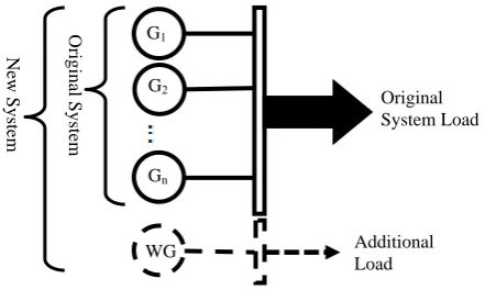
2.1 Computing ELCC for Conventional Units We start by considering a system with n conventional units. Ignoring transmission constraints, the system can be represented by a single node model as shown in Fig. 1.
The total system generation capacity should exceed the load level to maintain certain LOLP. The maximum load that can be supplied by the generating units is assumed to be L when the LOLP index satisfies the * system reliability criteria ( *
LOLP ). The value of the * L can be determined by solving the following
G1
G2
Gn
WG Additional
Load
Ne
w Syst
em
O
riginal System
Fig. 1 new system with added wind generator.
Original System Load
optimization problem:
Max(L)
subject to
*i
LOLP(L, C) LOLP
L G
≤
≤
∑
(1)
where, Gi is the capacity of the i-th unit. The second inequality constraint represents the upper bound on the system load. In a realistic case, when the generating units are not perfect, this constraint is not active and the first constraint determines the optimum value of the load. The LOLP can be calculated using the equivalent load duration curve (ELDC) [21]. Hence,
* *
C
LOLP =f (L ) (2)
where, fC indicates the risk function [21]. In a system with conventional generators, fC can be calculated using the following convolution process:
new
* *
C C C
*
C new
f (L ) (1 FOR) f (L )
FOR f (L C )
+ = − ×
+ × −
(3)
where, *
L and C are the original system load and capacity, respectively, and Cnew denotes the capacity of
the newly added unit. When the original system is at its optimum level, the newly added unit should carry the extra load. This is the concept of the effective load carrying capacity (ELCC). Accordingly,
new
1 * 1 *
C C C
ELCC=f−+ (LOLP ) f (LOLP )− − (4)
2.2 Difference between WTG and CG
Due to the stochastic nature of the wind speed, modeling of the wind turbine generators (WTG) is a quite complex task. Furthermore, there are some degrees of correlation between the wind speed and system load, which affect the WTG’s ELCC. Therefore, the convolution method cannot be applied on at a system including the WTGs. It is not possible to derive a closed form solution for the ELCC in this situation. However, the Monte Carlo approach can be used for the numerical analysis, considering the load and wind correlation. In this circumstance, the ELCC calculation problem can be rewritten as the following optimization problem:
Max(L)
* *
new
subject to LOLP(L + ΔL, C C+ )≤LOLP (5)
where, ΔL, is load increment and Cnew indicates increase in the system capacity due to the wind generators. According to its concept, the ELCC is implicitly equal to the ΔL.
Now, the main problem is how to present the wind speed and load model and their correlation in the Monte Carlo approach. The correlation can be positive or negative and its extents differ from site to site. In the practical calculation of the ELCC, the dependency
between the load and wind are merged into the historical data to implicitly consider the effect of the WLC. However, the obtained result is case dependent and cannot be used for general conclusions. In this paper, the correlation coefficient is changed in the copula models. Hence, different types of the WLC are modeled for possible situations.
To analyze the impact of the WLC on the ELCC of the WTG, the aim is to use a proper method which is able to consider the WLC explicitly. The copula technique is an appropriate method for this purpose. Before presenting the copula method, the wind and load models are introduced in the next section.
3 Wind and Load model
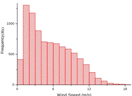
3.1 Wind Speed and Wind Generation Modeling Wind speed can be modeled using Wiebull, gamma, log-normal or burr distributions [11]. In this study, the wind speed data, recorded in Afriz area, Khorasan province, Iran in 2007 and 2008, are used to derive the model. For this data, the wind speed distribution is shown in Fig. 2. The wind power values have been calculated based on the hourly wind speed data, using the turbine’s power curve. Typical pitch-controlled wind turbine generators (WTG) are considered in this study. A linear WTG power curve is represented in [20] and the wind generation is obtained based on the method described in [19]. The wind turbine power curve has been modeled based on a two-MW VETAS V100 turbine [22]. As the wind speed regime is assumed to be identical for all wind turbines in a wind farm, the total generated power of the wind farm is obtained by aggregating the generations of all wind turbines.
3.2 Load Modeling
Annual hourly load curve data in Khorasan province in Iran have been shown in Fig. 3. These data have been collected from a bus near Khaf, over a one year period starting from May 20th, 2011.
0 6 12 18
0 500 1000
F
re
que
nc
y
W ind Speed (m/s)
Fig. 2 Wind Speed Data Histogram.
(Hz)
0 20000 40000 0
600 1200 1800
Frequ
ency
Load (KW)
Fig. 3 load histogram for annual empirical data in Khaf.
0 8 16
10000 20000 30000
L
oad
(
K
W
)
Wind Speed (m/s)
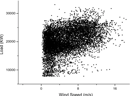
Fig. 4 Scatter plot for Load Samples and Wind Speed shows their correlation.
The Load is usually modeled based on the Gaussian distribution [23] in which the forecasting error is represented. This method is very useful and practical in short-term simulations. In the long-term, however, the Gaussian distribution cannot be utilized for load modeling. In this case, load distribution is close to a normal distribution with a skewed to the left side. Hence, the load marginal distribution should be derived from the historical data of the system. In [24] and [25] a kernel method has been presented for load modeling using the actual data. In this paper, the empirical distribution function is used for the load data as well as the wind data.
4 Wind Speed and Load Correlation Modeling The marginal distribution of the wind speed and load samples was shown in the previous section. The scatter plot for the wind speed and load samples is shown on Fig. 4. This figure indicates the correlation between the wind speed and load with the correlation degree of 0.4056.
In many cases, the modeling has been done based on the assumption of independence between these variables. But in some cases the variables are dependent. Different methods have been proposed for modeling such dependency. Choleskey transformation is one of the most commonly used methods [26] which is used in the multivariable normal distributions.
Complexity arises when the variables with different Probability Distribution Function (PDF) are correlated, e.g. the correlation between the wind speed and load. For modeling the correlation between wind speed and load, the Copula technique can be used. This technique is based on the Sklar’s theorem [19]. By this theorem, the marginal distributions F (x )i i can be joined together by a Copula function, C, and to produce a joint cumulative distribution function F (x , x ,..., x )c 1 2 n :
(6)
c 1 2 n 1 1 2 2 n n
F (x , x ,..., x )=C(F (x ), F (x ),..., F (x ))
In other words, C can be interpreted as a transformation on the marginal CDF of the corresponding random variables to form the joint CDF. By substituting (F (x ), F (x ),..., F (x ))1 1 2 2 n n with
1 2 n
(U , U ,..., U ), (6) can be rewritten as,
(7)
c 1 2 n 1 2 n
F (x , x ,..., x )=C(U , U ,..., U )
where, Ui is the marginal CDF of the i-th variable. In case of different distributions of the variables, a Copula function can merge them together to generate their joint cumulative distribution function. ‘Gaussian’ and ‘t’ copulas are two well-known Copulas, reported in the literature, with the similar behaviors. Multivariable t-distribution has good performances in tail data modeling. The t-copula CDF is given by [27]:
(7)
1 1
1 2
1 2 n
1
1 2
t ( U ) t ( U )
2 C(U , U ,..., U )
1
( )
X P X 2
... 1 dX
( ) ( ) P 2
− −
ν ν
ν+ −
−∞ −∞
= ν +
Γ ⎛ ′ ⎞
+
⎜ ⎟
ν ⎝ ν ⎠
Γ πν
∫
∫
where, ν is the degree of freedom, determined from the data processing. As the ν increase, the t-distribution approaches to the normal distribution.is In (8), the upper limit of the integrations, 1
1 t (u )−
ν , represents the inverse
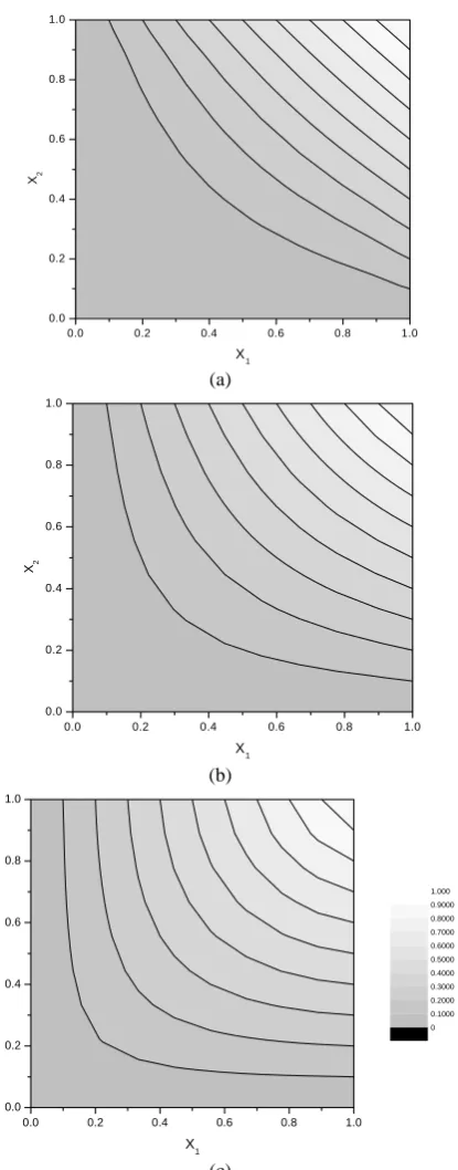
CDF of standard t-distribution and P is linear correlation matrix. In bivariate case, the correlation coefficient is the off-diagonal element of the correlation matrix. By changing this parameter, the correlation between X samples is changed. The contour plot for a bivariate standard t-copula CDF has been plotted in Fig. 5 with different correlation degrees.
With the help of the inverse copula function, one dimension joint CDF samples can be transformed into a bivariate or multivariate marginal CDF. By identifying the inverse marginal CDF, the correlated samples can be generated. Copula functions separate the correlation structure from the marginal distribution [28].
(Hz)
0.0 0.2 0.4 0.6 0.8 1.0 0.0
0.2 0.4 0.6 0.8 1.0
X1 X2
(a)
0.0 0.2 0.4 0.6 0.8 1.0
0.0 0.2 0.4 0.6 0.8 1.0
X1 X2
(b)
0.0 0.2 0.4 0.6 0.8 1.0
0.0 0.2 0.4 0.6 0.8 1.0
X1 X2
0 0.1000 0.2000 0.3000 0.4000 0.5000 0.6000 0.7000 0.8000 0.9000 1.000
(c)
Fig. 5 t-Copula CDF for correlation coefficient (a) -0.5, (b) 0 and (c) 0.5.
Any marginal distribution function, e.g. Wiebull and normal distributions, can be used to generate the joint distribution. In empirical studies, the marginal distribution can be extracted from the real data and used in the copula modeling approach. In Fig. 6 copula method is used to model the actual wind and load samples. The correlation coefficient in copula function is adjusted based on actual data, which is around 0.4.
0 8 16
10000 20000 30000
Load (
K
W
)
W ind Speed (m /s)
Fig. 6 Simulated Samples for correlation coefficient 0.4.
0 8 16
10000 20000 30000
Lo
ad (K
W)
W ind Speed (m /s)
(a)
0 8 1 6
10 0 00 20 0 00 30 0 00
L
oad (K
W)
W in d S p e e d (m /s)
(b)
0 8 16
10000 20000 30000
L
oad
(
K
W)
W ind S peed (m /s)
(c)
Fig. 7 Simulated Samples for correlation coefficient (a) -0.5, (b) 0 and (c) 0.5.
Comparison between Figs. 6 and 4 confirms that the copula modeling can sufficiently represent the actual behavior of the wind speed and load. These samples tested by the paired-sample Kolmogorov-Smirnov test which is a statistical test used to determine whether two sets of data arise from the same or different distributions. The test method has been presented in [29]. By changing the correlation coefficient, different sets of the samples can be generated. In Fig. 7, three different scenarios for the wind speed and load correlation (0.5, 0 and -0.5) have been simulated. These simulations have been conducted with the help of Copula CDF functions, shown in Fig. 5.
5 Case Study and Simulation
To evaluate the proposed method, the RBTS is used in this paper [30]. The single line diagram of the test system is shown in Fig. 8. The original RBTS has five different conventional units, with the total generation capacity of 240 MW, and the system peak load of 185 MW. In this paper, it is assumed that the load at buses are fully correlated with the same load distributions. The Load distribution is considered to be same as the distribution presented in section 3.1. It is a simplifying assumption to reduce the calculation cost. The wind speed distribution is obtained based on the data described in section 3.2. The correlation for these sets of samples is adjusted to generate different scenarios, based on the method described in section 4. The accuracy of the simulation depends on the WLC modeling which has been addressed by the copula modeling approach in this paper. Two different reliability indices are used in this paper, including the LOLP and the EENS.
6 Simulation Result
In this section, three different WTGs with the capacity of 10, 20 and 30 MW are added to bus #2 in the original test system. As the effect of the correlation coefficients on the system reliability indices is the main concern in this section, the WTGs’ FOR is set to zero for the simplicity in analysis of the system behavior.
For each WTG, the correlation with the load is changed in the model and the effect is compared. The obtained results are based on 10000 samples. MCS samples for a given accuracy level is independent of system size [31]. For relaxing some computational burdens, samples are discretized in eight steps. Similar to [4], branches and transmission network are considered to be fully reliable. All possible combinations of the conventional generator’s status, up to three outages, are considered at each step.
6.1 Effect of WTG on System Reliability Indices It is obvious that adding a generating unit will improve system reliability. For conventional units, this improvement is related to the unit size and FOR, but the advantage of WTGs is adversely affected by the wind speed probability and its correlation with the load.
Fig. 8 Single Line Diagram of the RBTS.
-0.6 -0.4 -0.2 0.0 0.2 0.4 0.6 0.8
6 12 18
EENS (MW
h
/yr)
C orrelation C oefficient 0 M W
10 M W 20 M W 30 M W
(a)
-0.6 -0.4 -0.2 0.0 0.2 0.4 0.6 0.8
0.00007 0.00014 0.00021
LOL
P
(Oc
c
/y
r)
C o rre la tio n C o e fficie n t 0 M W
1 0 M W 2 0 M W 3 0 M W
(b)
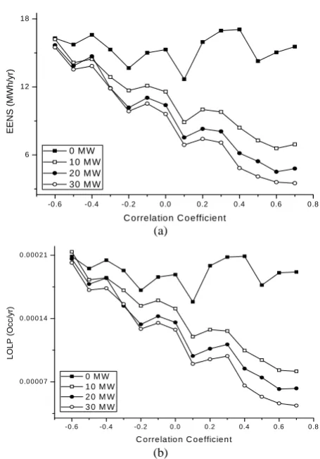
Fig. 9 Relibility Indices vs Correlation Degree for RBTS Associated with WTGs (a: EENS, b: LOLP).
Obviously, high correlated wind speed and load, indicate more generated power in the peak load period, which decreases the risk of the loss of load. This is confirmed by the downward trend in the system EENS, shown in Fig. 9, where EENS decreases with a higher correlation degree. In case of zero-MW WTG (no wind power generation), the LOLP and EENS are expected to be constant.
However, the variations in Fig. 9 may be regarded as the uncertainty in load modeling. The average LOLP and EENS for this case are 4
1.9149 10× − and 15.3886 MWh/year, respectively. The negative correlation decreases the benefits of the WTG on the reliability indices. For the correlation coefficient of -0.6, the system experiences a small improvement in the reliability due to the WTG capacity increment.
With higher correlation coefficients, the reliability is improved. However, with the correlation more than +0.4, the capacity of wind generation is the main factor. In this case, it is similar to adding conventional units with specified FOR. In an unreal scenario, where wind speed and load are fully correlated (not dependent), the WTG could be modeled by a conventional unit. A conventional unit has full dependency on the load (and hence they are fully correlated).
6.2 ELCC Calculation for WTGs
To calculate the ELCC, the bus loads are increased until the reliability indices return to the original system’s values.
-5 0 5 10 15 20 25 30
0 50 100 150
EE
NS (MW
h
/yr)
dL (M W ) -0.4
0 0.4 0.6
System with no W TG
0.0000 5.4054 10.8108 16.2162
dL (% of Peak Load)
(a)
0 10 20 30
0.0000 0.0005 0.0010 0.0015
LOLP (
O
CC
/yr)
dL (MW ) -0.4
0 0.4 0.6
System with no W TG
0.0000 5.4054 10.8108 16.2162
dL (% of Peak Load)
(b)
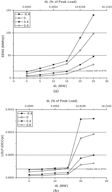
Fig. 10 Relibility Indices changes by load increment in different wind – load correlation (a) EENS (b) LOLP
Table 1 ELCC for different correlation coefficient.
Correlation Coefficient
Based on EENS index
Based on LOLP index
-0.50 1.29 6.38 -0.40 1.04 5.80 -0.30 2.83 11.25 -0.20 5.19 15.15 -0.10 5.06 15.08 0.00 5.01 12.92 0.10 10.03 15.56 0.20 10.23 15.45 0.30 10.01 15.48 0.40 15.30 16.27 0.50 17.49 17.57 0.60 18.14 17.74 0.70 21.40 20.18
Peak load value in buses 2 through 6 has been increased by 1 MW steps. In other words, the system peak load has increased by 5 MW steps. In each step, the system indices are recalculated and compared to their original values. Incremental changes in the EENS and LOLP indices are shown in Fig. 10, respectively, for a 30-MW WTG.
As mentioned in section 2.2, the ELCC equals to the load value added to the system and restores the system reliability indices back to their original values (i.e. maintains a constant level of LOLP and EENS). The EENS and LOLP Indices can be used for the ELCC calculation [4]. The ELCC is obtained when these indices are equal to the original system values. The ELCC values, calculated by the interpolation based on EENS and LOLP separately, are presented in Table 1.
The results of Table 1 are also is shown in Fig. 11. As it shown in Fig. 11, in case of negative correlation, use of the LOLP index for the ELCC calculation is optimistic. In case of the negative correlation, the peak system load cannot be served. With higher correlation degrees, more wind energy is injected during the peak load interval as demonstrated by Fig. 11, where two curves, obtained based on the LOLP and EENS indices, converge together.
-0.6 0 .0 0.6
0 8 16 24
EL
CC
(
M
W
)
C orre lation C o e fficie nt
B ase d on E E N S in de x B ase d on L O L P in de x
0 .0000 4 .3244 8 .6488 1 2.973 2
E
L
C
C
(%
of
P
e
a
k
Lo
ad
)
Fig. 11 ELCC vs. Correlation degree in RTBS Associated with 30 MW WTG.
7 Conclusion
This paper proposed a method for modeling wind speed and load correlation in order to analyze the effect of the wind speed and load correlation on the WTG’s ELCC. Due to the different marginal distributions of the wind speed and load and non-linear correlation between them, common methods such as joint normal or Choleskey transformation cannot be applied properly to this problem. Hence, in this paper the Copula and Monte Carlo techniques were employed for modeling on the wind speed and load correlation. As the main contribution of this paper, the copula modeling technique was employed to generate the joint distribution functions from the known marginal distribution functions such as, Wiebull or normal distribution. However, the empirical distributions can be directly used for the historical data. It was shown that the proposed method is able to simulate different scenarios and can be used for various case studies. Considering the mathematical and statistical basis and rich academic and empirical researches on the copula functions and modelling, this method can be optimized for better performance in the specified cases.
In this paper, different types of the correlation between load and wind speed was modeled. In the simulation study on the RBTS, having added a WTG to the system and adjusted the load and wind speed correlation, the ELCC was calculated based on maintaining a constant level of the EENS and LOLP. The simulation results clearly indicated the importance of the correlation coefficient between load and wind speed. This was demonstrated in the ELCC calculation for the WTGs. The result showed the ELCC is quite different when the correlation between wind speed and load is changed. This issue should be considered by the power system planners in wind energy deployment and WTG placement problems.
References
[1] S. Jadid and S. A. Bahreyni, “A Stochastic Planning Model for Smart Power Systems”,
Iranian Journal of Electrical & Electronic Engineering, Vol. 10, No. 4, pp. 293-303, 2014 [2] V. Koritarov, “Modeling Wind Energy
Resources in Generation Expansion Models”,
FERC Technical Conference on Planning Models and Software, Washington, DC, 2010. [3] Y. Ding, P. Wang, L. Goel, P. C. Loh and Q.
Wu, “Long-Term Reserve Expansion of Power Systems With High Wind Power Penetration Using Universal Generating Function Methods”,
IEEE Transactions on Power Systems, Vol. 26, No. 2, pp. 766-774, 2011.
[4] W. Wangdee and R. Billinton, “Considering Load-Carrying Capability and Wind Speed Correlation of WECS in Generation Adequacy Assessment”, IEEE Transactions on Energy
Converson, Vol. 21, No. 3, pp. 734-741, 2006. [5] Y. Gao, and R. Billinton, “Adequacy assessment
of generating systems containing wind power considering wind speed correlation”, Renewable Power Generation, IET , Vol.3, No.2, pp.217-226, 2009.
[6] B. Martin and J. Carlin, “Wind-Load Correlation and Estimates of the Capacity Credit of Wind Power: An Emprical Investigation”,
Wind Engineering, Vol. 7, No. 2, pp. 79-84, 1983.
[7] J. Haslett and M. Diesendorf, “The Capacity Credit of Wind Power: A Theoretical Analysis”,
Solar Energy, Vol. 26, No. 5, pp. 391-401, 1981.
[8] A. J. M. van Wijk, N. Halberg and W. C. Turkenburg, “Capacity credit of wind power in the Netherlands”, Electric Power Systems Research, Vol. 23, No. 3, pp. 189-200, 1992. [9] K. Coughlin and J. H. Eto, “Analysis of Wind
Power and Load Data at Multiple Time Scales”,
Ernest Orlando Lawrence Berkeley National Laboratory, Berkeley, 2010.
[10] L. Baringo and A. Conejo, “Correlated Wind-Power Production and Electric Load Scenarios for Investment Decisions”, Applied Energy, Vol. 101, pp. 475-482, 2013.
[11] Z. Qin, W. Li and X. Xiong, “Incorporating multiple correlations among wind speeds, photovoltaic powers and bus loads in composite system reliability evaluation.” Applied Energy, Vol. 110, pp. 285-294, 2013.
[12] E. P. Kahn, “Effective Load Carrying Capability of Wind Generation: Initial Results with Public Data”, The Electricity Journal, Vol. 17, No. 10, pp. 85–95, 2004.
[13] R. e. a. Zavadil, “Minnesota Public Utilities Commission statewide wind integration study”,
New York State Energy Research and Development Authority (NYSERDA), 2006. [14] k. Clark, G. Jordan, N. Miller and R. Piwko,
“The effects of integrating wind power on transmission system planning, reliability and operations”, New York State Energy Research and Development Authority (NYSERDA), 2005. [15] “Impact of Wind Power Generation In Ireland
on the Operation of Conventional Plant and the Economic Implications”, ESB National Grid, 2004.
[16] M. George, “Analysis of the power system impacts and value of wind power”,
International Journal of Engineering, Science and Technology, Vol. 3, No. 5, pp. 46-58, 2011. [17] G. Papaefthymiou, “Integration of Stochastic
Generation in Power Systems”, Delft University of Technology, Delft, Netherlands, 2007.
[18] G. Papaefthymiou and D. Kurowicka, “Using Copulas for Modeling Stochastic Dependencein Power System Uncertainty Analysis”, IEEE Transactions on Power Systems, Vol. 24, No. 1, pp. 40-49, 2009.
[19] S. Hagspiel, A. Papaemannouil, M. Schmid and G. Andersson, “Copula-based modeling of stochastic wind power in Europe and implications for the Swiss power grid”, Applied Energy, Vol. 96, pp. 33-44, 2011.
[20] H. Valizadeh Haghi, M. Tavakoli Bina, M. Golkar and S. Moghaddas-Tafreshi, “Using Copulas for analysis of large datasets in renewable distributed generation: PV and wind power integration in Iran”, Renewable Energy,
Vol. 35, No. 9, pp. 1991-2000, 2010.
[21] X. Wng and J. R. McDonald, Modern Power System Planning, New York: McGrw-Hill, 1984.
[22] vetas,[Online].Available:http://vestas.com/en/pr oducts_and_services/turbines/v100-2_0_mw. [Accessed Feb. 2014].
[23] S. M. Eslami, H. Rajabi Mashhadi and H. Modir Shanechi, “Effects of Wind Speed Forecasting Error on Control Performance Standard Index.”
Iranian Journal of Electrical & Electronic Engineering, Vol. 10, No. 3, pp. 223-229, 2014 [24] Z. Guo, W. Li, A. Lau, T. Inga-Rojas and K
Wang, “Detecting X-Outliers in Load Curve Data in Power Systems”, IEEE Transactions on Power Systems, Vol.27, No.2, pp.875-884, May 2012.
[25] J. Chen, W. Li, A. Lau, J. Cao and K. Wang, “Automated Load Curve Data Cleansing in Power Systems”, IEEE Transactions on Smart Grid, Vol.1, No.2, pp.213-221, Sep. 2010. [26] J. M. Morales, L. Baringo, A. J. Conejo and R.
Mı´nguez, “Probabilistic Power Flow with Correlated Wind Source”, IET Generation, Transmission & Distribution, Vol. 4, No. 5, pp. 641-651, 2010.
[27] S. Demarta and A. J. McNeil, “The t copula and related copulas”, International Statistical Review, Vol. 73, No. 1, pp. 111-129, 2005.
[28] R. B. Nelsen, An Introduction to Copulas, New York: Springer, 1999.
[29] J. A. Peacock, “Two-dimensional goodness-of-fit testing in astronomy”, Monthly Notices Royal Astronomy Society, Vol. 202, pp. 615-627. 1983.
[30] R. Billinton and e. al, “A Reliability Test System for Educational Purposes - Basic Data”, IEEE Transactions on Power Systems, Vol. 4, No. 3, pp. 1238-1244, 1989.
[31] M. Esmaili, H. A. Shayanfar and N. Amjady, “Stochastic Congestion Management Considering Power System Uncertainties”, Iranian Journal of Electrical & Electronic Engineering, Vol. 6, No. 1, pp. 36-47, 2010.
Mohammad Azim Armin was born in Bandarabbas, Iran, in 1981. He received the B.Sc. degree from Chamran University, Ahvaz, Iran, in 2004 and the M.Sc. degree from Ferdowsi University of Mashhad, Mashhad, Iran, in 2007, both in electrical engineering. He is Ph.D student in Ferdowsi University of Mashhad, Mashhad. His areas of interest include renewable power generation, system reliability evaluation and probabilistic load flow.
Habib Rajabi Mashhadi was born in Mashhad, Iran, in 1967. He received the B.Sc. and M.Sc. degrees with honor from the Ferdowsi University of Mashhad, both in electrical engineering, and the Ph.D. degree from the Department of Electrical and Computer Engineering of Tehran University, Tehran, Iran, under joint cooperation of Aachen University of Technology, Germany, in 2002. He is as Associate Professor of electrical engineering at Ferdowsi University of Mashhad. His research interests are power system operation and planning, power system economics, and biological computation.