Please cite this article as: M. Fallah, R. Tavakkoli-Moghadam, A.R. Salamatbakhsh-Varjovi, M. Alinaghian, A Green Competitive Vehicle Routing Problem under Uncertainty Solved by an Improved Differential Evolution Algorithm, International Journal of Engineering (IJE), IJE TRANSACTIONS A: Basics Vol. 32, No. 7, (July 2019) 976-981
International Journal of Engineering
J o u r n a l H o m e p a g e : w w w . i j e . i rA Green Competitive Vehicle Routing Problem under Uncertainty Solved by an
Improved Differential Evolution Algorithm
M. Fallaha, R. Tavakkoli-Moghaddam*b,c, A. Salamatbakhsh-Varjovid, M. Alinaghiane
a Department of Industrial Engineering, Tehran Central Branch, Islamic Azad University, Tehran, Iran b School of Industrial Engineering, College of Engineering, University of Tehran, Tehran, Iran c Arts et Métiers ParisTech, LCFC, Metz, France
d Department of Industrial Engineering, Science and Research Branch, Islamic Azad University, Tehran, Iran e Department of Industrial and Systems Engineering, Isfahan University of Technology, Isfahan, Iran
P A P E R I N F O
Paper history: Received 03 February 2019
Received in revised form 19 March 2019 Accepted 21 April 2019
Keywords:
Competitive Environment Green Vehicle Routing Problem Time Windows
Uncertainty
A B S T R A C T
Regarding the development of distribution systems in the recent decades, fuel consumption of trucks has increased noticeably, which has a huge impact on greenhouse gas emissions. For this reason, the reduction of fuel consumption has been one of the most important research areas in the last decades. The aim of this paper is to propose a robust mathematical model for a variant of a vehicle routing problem (VRP) to optimize sales of distributers, in which the time of distributor service to customers is uncertain. T o solve the model precisely, the improved differential evolution (IDE) algorithm is used and obtained results were compared with the result of a particle swarm optimization (PSO) algorithm. The results indicate that the IDE algorithm is able to obtain better solutions in solving large -sized problems; however, the computational time is worse than PSO.
doi: 10.5829/ije.2019.32.07a.10
1. INTRODUCTION1
In recent years, by increasing large-scale greenhouse gases (GHG) emissions, the social cost of the governments have considerably increased [1]. Increasing of fuel consumption creates significant negative impacts on greenhouse gas emissions.
Research has shown that in the real competitiv e world, the decrease of the distribution cost (especially in fuel consumption) has affected on the operation cost. The distribution cost depends on many criteria and can be separated into two broad categories. The first one includes the load, speed, road status, fuel consumption rate (in any distance), fuel price, etc. that are directly related to the scheduling issues. The second category includes vehicle depreciation, maintenance an d repair costs, driver's wages, taxes, etc. [2–5].
Tavakkoli-Moghaddam et al. [6] considered a rival vehicle routing problem for the first time that maximize s
*Corresponding Author Email: [email protected] (R. T avakkoli-Moghadam)
algorithm (PSO) and simulated annealing (SA) algorithm [16, 17].
Innovations of this research are as follows: the servicing time of rivals is considered under uncertainty and instead of an expected starting service time, a set of scenarios are considered in the proposed model, and a robust model is used to maximize the rate of sales and reduce the cost. In addition, reducing fuel consumption to reduce the operational cost and the harmful effects of greenhouse gases (especially, carbon and carbon dioxide) is also considered as bi-objectives. Moreover, a meta-heuristic based on IDE algorithm to find optimal solutions is another contribution used in this paper.
2. PROBLEM DEFINITION AND MODELING
2. 1. Collections And Indices AVRP can be indicated by a graph G = (S, A), such that the points of nodes and 𝑠 = {𝑖|𝑖 = 0, … , 𝑛} so that G is a set of the arrows and nodes; 𝐴 = {(𝑆𝑖, 𝑆𝑗): 𝑖 ≠ 𝑗} that is a set of nodes joining the arrows, and S0 represents the source. Dij≥0, which is denoted arc (i, j), indicates the distance or
cost of traveling among the two nodes i and j. The parameters used in this model are presented as follows :
N Number of customers (i and j are the indices of customers)
𝑦𝑣 Number of vehicles 𝑘𝑦𝑣 The Capacity of vehicle v
𝑇𝑣 Upper bound of the travel time of vehicle v.
𝑇𝑣 Demand of the nodei.
𝑡𝑖𝑗𝑣 Time travel from node i to node j by vehicle v
M large number
𝑑𝑡𝑑𝑖 Time dependent demand of customeri
𝑡𝑢𝑖𝑠 In scenario s, an upper limit of rivals arrival time to node i
𝑡𝑙𝑖𝑠 In scenario s, a lower limit of rivals arrival time to node i
𝐷𝑖 Total i-th customer demand so that 𝐷𝑖= 𝑑𝑡𝑑𝑖+ 𝑑𝑖𝑛𝑖 𝐷𝑡𝑑𝑖 Demand of customer i (dependent to time)
𝐷𝑖𝑛𝑖 Demand of customer i (independent to time) 𝑐𝑜𝑟𝑟 Slip friction coefficient in each road
𝐶𝑒𝑑 Air resistance coefficient 𝐹𝑘 Front of the vehicle v
𝐴𝑑 The density of air 𝐺𝑅 Earth's gravitational force
𝜃𝑔𝑖𝑗 Average gradient of the road from node i to j
𝑎𝑐𝑘 Acceleration of vehicle v in meters per squared second
𝑤𝑣𝑘 Weight of vehicle v
𝑊𝑙 Load unit weight
𝑑𝑖𝑗 Distance between customers i and j 𝑣𝑘 Speed of vehicle v
𝑙𝑖 Amount of time when vehicle reaches node i 𝐷𝑖 Demand of customer i
𝑥𝑖𝑗𝑣 1, if vehicle v passes via route [𝑖, 𝑗]
𝑜𝑖𝑠 1, in scenario s, if the driver meets the customer more quickly than the lower bound of the rival
𝑞𝑖𝑠 1, in scenario s, if the driver meets the customer during the rival time period
𝑧𝑖𝑠 1, in scenario s, if the distributer begins customer service after the rival upper bound
𝑦𝑖𝑠 1, in scenario s, if the driver meets customer before the rival upper bound.
2. 2. Mathematical Model The proposed mathematical model is defined as follows:
Max 𝑍1= ∑𝑠∈Ω𝑝𝑠[∑𝑛𝑖=1(𝑜𝑖𝑠𝑑𝑡𝑑𝑖+
𝑞𝑖𝑠(𝑡𝑢𝑖𝑠−𝑡𝑖
𝑡𝑢𝑖𝑠−𝑡𝑙𝑖𝑠)𝑑𝑡𝑑𝑖)] + 𝜆 ∑𝑠∈Ω𝑝𝑠[(∑ (𝑜𝑖𝑠𝑑𝑡𝑑𝑖+
𝑛 𝑖=1
𝑞𝑖𝑠(𝑡𝑢𝑖𝑠−𝑡𝑖
𝑡𝑢𝑖𝑠−𝑡𝑙𝑖𝑠)𝑑𝑡𝑑𝑖) − ∑𝑠′∈Ω𝑝𝑠′[∑ (𝑜𝑖𝑠′𝑑𝑡𝑑𝑖+
𝑛 𝑖=1
𝑞𝑖𝑠′(
𝑡𝑢𝑖𝑠′−𝑡𝑖
𝑡𝑢𝑖𝑠′−𝑡𝑙𝑖𝑠′)𝑑𝑡𝑑𝑖)]) + 2𝜃𝑠] − 𝜔 ∑𝑠∈Ω𝑝𝑠𝛿𝑠
Min 𝑍2= ∑ ∑ ∑𝑛 (𝑓𝑘+ 𝑔𝑠𝑖𝑛𝜃𝑔𝑖𝑗+
𝑖=1 𝑛 𝑗=0 𝑦𝑣 𝑣=1
𝑔𝑟𝑐𝑜𝑟𝑟𝑐𝑜𝑠𝜃𝑔𝑖𝑗) (𝑤𝑣𝑘+ 𝑤𝑙𝑗𝑣)dij𝑥𝑖𝑗𝑣 +
∑𝑛𝑣𝑣=1∑𝑛𝑗=0∑𝑛𝑖=10.5𝑐𝑒𝑑 𝐴𝑐𝑘𝐴𝑑𝑣𝑘2dij𝑥𝑖𝑗𝑣
(1)
∑𝑛𝑖=1∑𝑦𝑣𝑣=1𝑥𝑖𝑗𝑣 = 1, ∀ 𝑗 = 2, … , 𝑛 (2)
∑𝑛𝑗=1∑𝑦𝑣𝑣=1𝑥𝑖𝑗𝑣 = 1, ∀𝑖 = 2, … , 𝑛 (3)
∑𝑛 𝑥𝑖𝑗𝑣
𝑖=1 =
∑𝑛 𝑥𝑗𝑖𝑣 ,
𝑖=1
∀ 𝑗 = 1,2, … , 𝑛 𝑣 =
1, … , 𝑦𝑣 (4)
(𝑙𝑖𝑣− 𝑑𝑖− 𝑙𝑗𝑣)𝑥𝑖𝑗𝑣= 0 ∀𝑖 = 0,1, … , 𝑛 𝑗 =1, … , 𝑛 𝑣 = 1, … , 𝑦𝑣 (5)
∑𝑛𝑖=1𝑠𝑖∑𝑛𝑗=1𝑥𝑖𝑗𝑣+
∑ ∑ 𝑑𝑖𝑗
𝑣𝑘
𝑛
𝑗=1 𝑥𝑖𝑗𝑣 ≤ 𝑛
𝑖=1
𝑇𝑣
∀ 𝑣 = 1, … , 𝑦𝑣 (6)
𝑡𝑗= ∑ 𝑡𝑖∑𝑦𝑣 𝑥𝑖𝑗𝑣 𝑣=1 𝑛
𝑖=1 +
∑ ∑ (𝑑𝑖𝑗
𝑣𝑘)
𝑦𝑣
𝑣=1 𝑥𝑖𝑗𝑣+ 𝑠𝑗 𝑛
𝑖=1 ∀ 𝑗 = 2, … , 𝑛
(7)
∑ (𝐷𝑖− 𝑑𝑡𝑑𝑖𝑧𝑖𝑠) ∑𝑛 𝑥𝑖𝑗𝑣 𝑗=1 𝑛
𝑖=1 −
𝛿𝑠≤ 𝑘𝑦𝑣
∀ 𝑣 =
1,2, … , 𝑦𝑣 𝑠𝜖Ω (8)
(𝑡𝑢𝑖𝑠− 𝑡𝑖) − 𝑀(𝑦𝑖) ≤ 0 𝑖 = 1,2, … , 𝑛, 𝑠 ∈Ω (9)
𝑧𝑖𝑠+ 𝑦𝑖𝑠= 1 𝑖 = 1,2, … , 𝑛 𝑠 ∈Ω (11)
(𝑡𝑢𝑖𝑠− 𝑡𝑖)+𝑀(1 − 𝑞𝑖𝑠) ≥ 0 𝑖 = 1,2, … , 𝑛 𝑠 ∈Ω (12)
(𝑡𝑙𝑖𝑠− 𝑡𝑖)+𝑀(1 − 𝑜𝑖𝑠) ≥ 0 𝑖 = 1,2, … , 𝑛 𝑠 ∈Ω (13)
(𝑡𝑙𝑖𝑠− 𝑡𝑖) + 𝑀𝜛𝑖𝑠≤ 0 𝑖 = 1,2, … , 𝑛 𝑠 ∈Ω (14)
𝑞𝑖𝑠+ 𝜛 = 1 𝑖 = 1,2, … , 𝑛 𝑠 ∈Ω (15)
∑𝑛𝑖=1(𝑜𝑖𝑠𝑑𝑡𝑑𝑖+
𝑞𝑖𝑠(𝑡𝑢𝑖𝑠−𝑡𝑖
𝑡𝑢𝑖𝑠−𝑡𝑙𝑖𝑠)𝑑𝑡𝑑𝑖) −
∑𝑠∈Ω𝑝𝑠(∑𝑛𝑖=1(𝑜𝑖𝑠𝑑𝑡𝑑𝑖+
𝑞𝑖𝑠(𝑡𝑢𝑖𝑠−𝑡𝑖
𝑡𝑢𝑖𝑠−𝑡𝑙𝑖𝑠)𝑑𝑡𝑑𝑖)) + 𝜃𝑠≥ 0
𝑠 ∈Ω (16)
∑ ∑ ∑ 𝑥𝑖𝑗𝑣
𝑗∉𝑆 𝑗∈𝑆 𝑛𝑣
𝑣=1 ≤ |𝑠| −
𝑝(𝑠) ∀ 𝑆 ⊆ 𝐴 − {1} 𝑠 ≠ϕ (17)
𝑥𝑖𝑗, 𝑜𝑖𝑠, 𝑦𝑖𝑠, 𝑧𝑖𝑠, 𝑞𝑖𝑠, 𝜛𝑖𝑠∈ [0,1] 𝑡𝑖≥ 0 𝑡1= 0 (18)
Equation (1) indicates the sales of distributer under uncertainty, and concerns reducing GHG emission and fuel consumption.
Restrictions (2) and (3) make it possible for each request to be served only from a distributor vehicle. Constraint (4) states that if a vehicle is to be inserted into a node, it must be removed, thus connecting the routes. Constraint (5) states that if 𝑥𝑖𝑗𝑣 = 1, the amount of goods
carried to the j-th node is equal to the load transferred to the i-th node minus the i-th node’s demand (i.e., the i-th node is served immediately by the i-th vehicle by the v -th vehicle immediately).
Constraint (6) indicates that the service time and route should be less than the specified value. Constraint (7) indicates the start time for serving customers. Constraints (8) to (11) indicates that if vehicle 𝑣 starts to serve in the scenarios earlier t han 𝑡𝑢𝑖𝑠 to customer 𝑖 then the i-th customer demand must be equal to 𝐷𝑖 from the base station. This is because the distributor starts service faster than other competitors do and can take all profitable business out of it. If the start-of-service time to the i-th customer is after 𝑡𝑢𝑖𝑠, then the profit previously earned will only be equal to the amount of independent demand. Constraints (12) to (15) relate to maximizing profits. Constraint (16) indicates the difference between the profits earned in the scenarios and expected value of earning profits for all scenarios. Cons traint (17) is related to the elimination of subtractions, and the Constraint (18) relates to the model variables.
3. PROBLEM-SOLVING APPROACH
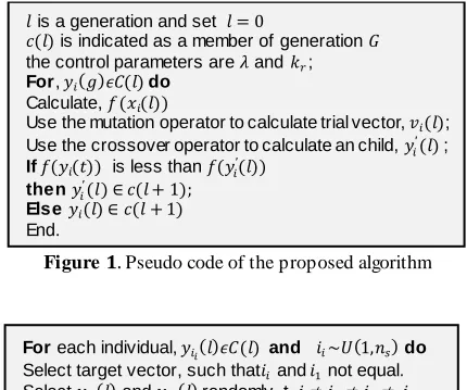
The differential evolution (DE) was first proposed by
Storn and Price [18]. Due to considerable performance in discrete problems, DE has been used in solving problems in the past years [19]. The proposed algorithm is shown in Figure 1.
To define mutation operator in DE, trial vector,
𝑣𝑖(l), for every individual of exciting population is
generated by mutating. Off spring vector is produced trial vector, 𝑣𝑖(l) by a crossover operator for parent yi(l). The trial vector 𝑣𝑖(l) is demonstrated in Figure 2.
Offspring vector, 𝑦𝑖′(𝑡), is generated by:
𝑦𝑖𝑘′(𝑡) = {𝑦𝑣𝑖𝑘(𝑙) if 𝑗 ∈ 𝛿
𝑖𝑘(𝑙) otherwise (19)
where 𝑦𝑖𝑘(𝑔) presents to the 𝑘-th (𝑘 ∈ {1, … , 𝑛𝑥})
particle of vector , 𝑦𝑖(𝑔), and a set of crossover points are represented as 𝛿. The DE binomial crossover operator is shown in Figure 3.
Experimental studies show that model
𝐷𝐸 𝑟𝑎𝑛𝑑⁄ ⁄ 𝑏𝑖𝑛1⁄ , in which a target vector is chosen
randomly, provides a good variety in answers and is capable of converging the answers. On the other hand, strategy 𝑐𝑢𝑟𝑟𝑒𝑛𝑡 − 𝑡𝑜 𝑏𝑒𝑠𝑡 2⁄ 𝑏𝑖𝑛⁄ will result in convergence in answers, which is shown in the following equation:
𝑣𝑖(𝑔) = 𝑦𝑖1(𝑔) + 𝛽(𝑦̂(𝑔) − 𝑦𝑖(𝑔)) + 𝛽(𝑦𝑖2(𝑔) −
𝑦𝑖3(𝑔))
(20)
where a differential vector is first calculated from the difference between best available vector 𝑦̂(𝑔) with parent vector 𝑦𝑖(𝑔) and the second differential vector is calculated by the difference between 𝑦𝑖2(𝑔), 𝑦𝑖3(𝑔) vectors which are chosen randomly to achieve the best results in DE, strategies are used dynamically based on
Figure 1. Pseudo code of the proposed algorithm
Figure 2. Selecting trial vector by the mutation
𝑙 is a generation and set 𝑙 = 0
𝑐(𝑙) is indicated as a member of generation 𝐺
the control parameters are 𝜆 and 𝑘𝑟;
For, 𝑦𝑖(𝑔)𝜖𝐶(𝑙)do
Calculate, 𝑓(𝑥𝑖(𝑙))
Use the mutation operator to calculate trial vector, 𝑣𝑖(𝑙);
Use the crossover operator to calculate an child, 𝑦𝑖′(𝑙) ; If 𝑓(𝑦𝑖(𝑡)) is less than 𝑓(𝑦𝑖′(𝑙))
then𝑦𝑖′(𝑙) ∈𝑐(𝑙 + 1); Else 𝑦𝑖(𝑙) ∈𝑐(𝑙 + 1)
End.
For each individual, 𝑦𝑖𝑖(𝑙)𝜖𝐶(𝑙) and 𝑖𝑖~𝑈(1,𝑛𝑠)do
Select target vector, such that𝑖𝑖 and 𝑖1 not equal.
Select 𝑦𝑖2(𝑙) and 𝑦𝑖3(𝑙) randomly, t 𝑖 ≠ 𝑖1≠ 𝑖2≠ 𝑖3.
Calculate trial vector ass follow ing equation: 𝑣𝑖(𝑙) = 𝑦𝑖1(𝑡) + 𝜆(𝑦𝑖2(𝑔) − 𝑦𝑖2(𝑔))
Figure 3. DE binomial crossover operator
probability. 𝑑𝑠,1 and 𝑑𝑠,2= 1 − 𝑑𝑠,1are assumed as the probable selection of strategy DE rand⁄ ⁄ bin1⁄ and
DE current − to best⁄ ⁄ bin2⁄ , respectively as the
following equation:
𝑑𝑠,1=𝑞(𝑞𝑠,2+𝑞𝑞𝑠,1𝑓,2(𝑞)+𝑞𝑠,2+𝑞𝑠,2(𝑞𝑓,2𝑠,1)+𝑞𝑓,1) (21)
where 𝑞𝑠,1 and 𝑞𝑠,2 in next repetition 𝑐(𝑔 + 1), indicates children number 𝑦𝑖′(𝑔) which are considered according
to DE rand⁄ ⁄ bin1⁄ and DE current − to best⁄ ⁄ bin2⁄
respectively. Also, qf,1and qf,2 are the number of children which are not converted to the next repetition.
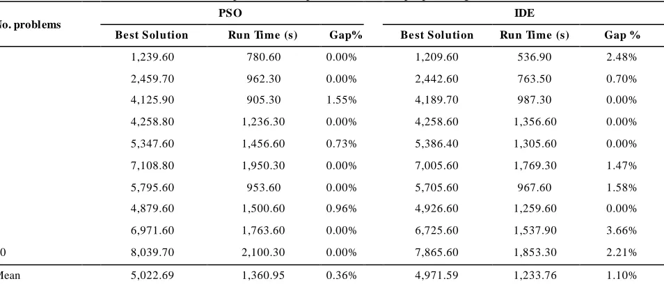
4. COMPUTATIONAL RESULTS
In this paper, standard samples of the PVRPTW considered by Cordeau et al. [20] are used. For each scenario, lower and upper bound of time windows are considered as upper and lower reaching times of vehicles. That is the upper limit of reaching time to customers is considered in all scenarios 𝑡𝑢𝑖𝑠 in a uniform distribution in interval [15, 60] and the lower limit of the distributors’ reaching time to customers in all scenarios 𝑡𝑙𝑖𝑠 in a uniform distribution in interval [10, 40].
The performance of algorithms is demonstrated in Table 1. In terms of the quality, IDE algorithm's solution
could improve an average of more than 1% of the solutions. The mean error for the IDE and PSO algorithms is 0.36 and 1.1%, respectively. The greatest improvement in IDE solution algorithm occurred in problem 9, and a 3.66% improvement in response has occurred. The average run time for PSO is lower than the IDE. On average, the PSO algorithm has a run time of PSO algorithm 1,233 seconds, which is about 10% less than the IDE resolution time.
5. CONCLUSION AND FUTURE RESEARCH
This paper has presented a robust mathematical model for a variant of a vehicle routing problem (VRP), in which a competition exists among distributors in order to increase their sales under uncertainty of customers by rivals. In addition, optimization of fuel consumption is related to decline of the effects of CO2. A set of scenarios for service time of distributers has been defined and optimized the objective function. Because of the computational complexity of the problem considered in this paper, two meta-heuristic algorithms (i.e., IDE and PSO) have been used and their performances were evaluated. The results indicate that IDE has better performance in terms of the results than PSO with more computational time in solving large-sized problems. For further studies, the demand for customers in an uncertain condition is proposed. Considering a competitive environment in other modes of the VRP may be an innovative topic for future research. Finally , implementation of the presented model, taking into account the actual data from a case study can be considered as one of the future studies.
TABLE 1. Comparison of the performance of the proposed algorithms
IDE PSO
No. problems
Gap % Run Time (s)
Be st Solution Gap%
Run Time (s) Be st Solution
2.48% 536.90
1,209.60 0.00%
780.60 1,239.60
1
0.70% 763.50
2,442.60 0.00%
962.30 2,459.70
2
0.00% 987.30
4,189.70 1.55%
905.30 4,125.90
3
0.00% 1,356.60
4,258.60 0.00%
1,236.30 4,258.80
4
0.00% 1,305.60
5,386.40 0.73%
1,456.60 5,347.60
5
1.47% 1,769.30
7,005.60 0.00%
1,950.30 7,108.80
6
1.58% 967.60
5,705.60 0.00%
953.60 5,795.60
7
0.00% 1,259.60
4,926.60 0.96%
1,500.60 4,879.60
8
3.66% 1,537.90
6,725.60 0.00%
1,763.60 6,971.60
9
2.21% 1,853.30
7,865.60 0.00%
2,100.30 8,039.70
10
1.10% 1,233.76
4,971.59 0.36%
1,360.95 5,022.69
Mean
Select 𝛿~𝑈(1, 𝑛𝑠)and 𝑝𝑟 randomly.
Foreach𝑗, 𝑦𝑖(𝑙)
If𝑘𝑟> 𝑈(0,1) then 𝛿 ← 𝛿 ∪ {𝑗}
6. REFERENCES
1. Fallah, M., Mohajeri, A. and Barzegar-Mohammadi, M., “A New Mathematical Model To Optimize A Green Gas Network: A Case Study”, International Journal of Engineering-Transactions A:
Basics, Vol. 30, No. 7, (2017), 1029–1037.
2. Sbihi, A. and Eglese, R.W., “Combinatorial optimization and green logistics”, Annals of Operations Research, Vol. 175, No. 1, (2010), 159–175.
3. Norouzi, N., Sadegh-Amalnick, M. and T avakkoli-Moghaddam, R., “Modified particle swarm optimization in a time-dependent vehicle routing problem: minimizing fuel consumption”,
Optimization Letters, Vol. 11, No. 1, (2017), 121–134.
4. Xiao, Y., Zhao, Q., Kaku, I. and Xu, Y., “Development of a fuel consumption optimization model for the capacitated vehicle routing problem”, Computers & Operations Research, Vol. 39, No. 7, (2012), 1419–1431.
5. Arab, R., Ghaderi, S.F. and T avakkoli-Moghaddam, R., “Solving a New Multi-objective Inventory-Routing Problem by a Non-dominated Sorting Genetic Algorithm”, International Journal of
Engineering-Transactions A: Basics, Vol. 31, No. 4, (2018),
588–596.
6. T avakkoli-Moghaddam, R., Gazanfari, M., Alinaghian, M., Salamatbakhsh, A. and Norouzi, N., “A new mathematical model for a competitive vehicle routing problem with time windows solved by simulated annealing”, Journal of manufacturing
systems, Vol. 30, No. 2, (2011), 83–92.
7. Norouzi, N., T avakkoli-Moghaddam, R., Ghazanfari, M., Alinaghian, M. and Salamatbakhsh, A., “A new multi-objective competitive open vehicle routing problem solved by particle swarm optimization”, Networks and Spatial Economics, Vol. 12, No. 4, (2012), 609–633.
8. Salamatbakhsh-Varjovi, A., T avakkoli-Moghaddam, R., Alinaghian, M. and Najafi, E., “Robust Periodic Vehicle Routing Problem with T ime Windows under Uncertainty: An Efficient Algorithm”, KSCE Journal of Civil Engineering, Vol. 22, No. 11, (2018), 4626–4634.
9. Erera, A.L., Morales, J.C. and Savelsbergh, M., “T he vehicle routing problem with stochastic demand and duration constraints”, Transportation Science, Vol. 44, No. 4, (2010), 474–492.
10. Qi, M., Qin, K., Zhao, Y. and Liu, J., “ A study of the vehicle scheduling problem for victim transportation”, International
Journal of Management Science and Engineering
Management, Vol. 8, No. 4, (2013), 276–282.
11. Goodson, J.C., Ohlmann, J.W. and Thomas, B.W., “ Cyclic-order neighborhoods with application to the vehicle routing problem with stochastic demand”, European Journal of Operational
Research, Vol. 217, No. 2, (2012), 312 –323.
12. Mulvey, J.M., Vanderbei, R.J. and Zenios, S.A., “ Robust optimization of large-scale systems”, Operations Research, Vol. 43, No. 2, (1995), 264–281.
13. Hamidieh, A., Arshadikhamseh, A. and Fazli-Khalaf, M., “A Robust Reliable Closed Loop Supply Chain Network Design under Uncertainty: A Case Study in Equipment T raining Centers”, International Journal of Engineering-Transactions
A: Basics, Vol. 31, No. 4, (2017), 648–658.
14. Lenstra, J.K. and Kan, A.R., “Complexity of vehicle routing and scheduling problems”, Networks, Vol. 11, No. 2, (1981), 221– 227.
15. Jia, H., Li, Y., Dong, B. and Ya, H., “An improved tabu search approach to vehicle routing problem”, Procedia-Social and
Behavioral Sciences, Vol. 96, (2013), 1208–1217.
16. Fazel Zarandi, M.H., Hemmati, A., Davari, S. and T urksen, I.B., “A simulated annealing algorithm for routing problems with fuzzy constrains”, Journal of Intelligent & Fuzzy Systems, Vol. 26, No. 6, (2014), 2649–2660.
17. Goksal, F.P., Karaoglan, I. and Altiparmak, F., “A hybrid discrete particle swarm optimization for vehicle routing problem with simultaneous pickup and delivery”, Computers & Industrial
Engineering, Vol. 65, No. 1, (2013), 39–53.
18. Storn, R. and Price, K., “ Differential evolution –a simple and efficient heuristic for global optimization over continuous spaces”, Journal of global optimization, Vol. 11, No. 4, (1997), 341–359.
19. Qin, A.K. and Suganthan, P.N., “ Self-adaptive differential evolution algorithm for numerical optimization”, In 2005 IEEE congress on evolut ionary computation, Vol. 2, IEEE, (2005), 1785–1791.
20. Cordeau, J.F., Gendreau, M. and Laporte, G., “ A tabu search heuristic for periodic and multi‐depot vehicle routing problems”,
Networks: An International Journal, Vol. 30, No. 2, (1997),
A Green Competitive Vehicle Routing Problem under Uncertainty Solved by an
Improved Differential Evolution Algorithm
M. Fallaha, R. Tavakkoli-Moghaddamb,c, A. Salamatbakhsh-Varjovid, M. Alinaghiane
a Department of Industrial Engineering, Tehran Central Branch, Islamic Azad University, Tehran, Iran b School of Industrial Engineering, College of Engineering, University of Tehran, Tehran, Iran c Arts et Métiers ParisTech, LCFC, Metz, France
d Department of Industrial Engineering, Science and Research Branch, Islamic Azad University, Tehran, Iran e Department of Industrial and Systems Engineering, Isfahan University of Technology, Isfahan, Iran
P A P E R I N F O
Paper history: Received 03 February 2019
Received in revised form 19 March 2019 Accepted 21 April 2019
Keywords:
Competitive Environment Green Vehicle Routing Problem Time Windows
Uncertainty
هدیکچ
لاس لوط رد نازیم شیازفا اب نامزمه ،هتشذگ یاه
متسیس ،اضاقت هتشاد یساسا تارییغت لااک عیزوت یاه
زیم اذل ،دنا فرصم نا
راشتنا و اوه یگدولآ رب یدایز ریثات یاراد هک تسا هتفای شیازفا یهجوت لباق روط هب زین هدننک عیزوت هیلقن طیاسو تخوس
هناخلگ یاهزاگ م زا دیدج یضایر لدم کی هئارا ،هلاقم نیا هئارا زا فده .دراد یا
هب هیلقن طیاسو یبایریسم هلاس
هنیمکروظنم هنیشیب و تخوس فرصم یزاس عیزوت نایم رد یتباقر طبارش رد بسک لباق دوس یزاس
تحت ناگدننک مدع طیارش
سیورس عورش تیعطق عیزوت یهد
هنیهب درکیور زا هدافتسا اب نایرتشم هب ناگدننک ا .تسا ویرانس تحت راوتسا یزاس
یوس ز
فرصم شهاک رگید هنیزه شهاک هب رجنم تخوس
یم هیلقن طیاسو یراج یاه سیورس عورش نامز شهاک و دوش
هب یهد
عیزوت ریاس اب هسیاقم رد شورف خرن شیازفا ثعاب نایرتشم یم یتباقر طیحم رد ناگدننک
ک یبایزرا روظنم هب .دوش لدم ییارا
ب و دش هدافتسا هتفای دوبهب یلضافت لماکت متیروگلا زا هدش هئارا متیروگلا درکلمع یبایزرا روظنم ه
یپ یاه یدادعت ،یداهنش
یتابساحم جیاتن .دش یسررب و هسیاقم تارذ هوبنا متیروگلا طسوت هلاسم لح جیاتن اب و داجیا گرزب داعبا رد هنومن هلاسم
یم ناشن لضافت لماکت متیروگلا هک دهد یم یرتهب یتابساحم یدرکلمع یاراد
وبنا متیروگلا اما ،دشاب نامز یاراد تارذ ه
یم یرتهب یتابساحم .دشاب