Modeling MOOC Student Behavior With Two-Layer Hidden Markov Models

Modeling MOOC Student Behavior With

Two-Layer Hidden Markov Models

Chase Geigle

Department of Computer Science University of Illinois (UIUC)

Urbana, Illinois, USA [email protected]

ChengXiang Zhai

Department of Computer Science University of Illinois (UIUC)

Urbana, Illinois, USA [email protected]

Massive open online courses (MOOCs) provide educators with an abundance of data describing how students interact with the platform, but this data is highly underutilized today. This is in part due to the lack of sophisticated tools to provide interpretable and actionable summaries of huge amounts of MOOC activity present in log data. To address this problem, we propose a student behavior representation method alongside a method for automatically discovering those student behavior patterns by leveraging the click log data that can be obtained from the MOOC platform itself. Specifically, we propose the use of a two-layer hidden Markov model (2L-HMM) to extract our desired behavior representation, and show that patterns extracted by such a 2L-HMM are interpretable and meaningful. We demonstrate that the proposed 2L-HMM can also be used to extract latent features from student behavioral data that correlate with educational outcomes.

1. I

The proliferation of massive open online courses (MOOCs) has resulted in a profound impact on education. As more and more students participate in these novel educational environments, it is of utmost importance that we be able to understand the behavioral patterns students exhibit in these environments. While we can easily observe the changes in behavior of students in real classrooms, MOOC environments present some significant challenges in this regard: the structure of the course itself is more hands-off in nature than that of the traditional classroom (in most cases), and thus attracts more students that are full-time workers with irregular learning schedules.

At the same time, this influx of learners turning to MOOC platforms to educate themselves directly leads to the collection of larger datasets of behavioral data through the platform’s logging. This presents a unique opportunity: the data present in these logs has the power to aid us in understanding the behavior of students who take our MOOCs. However, due to the vast scale of these behavioral logs, student behavior patterns are mostly undetectable for MOOC instructors and as a result, the rich data available through MOOC logs is highly underutilized today.

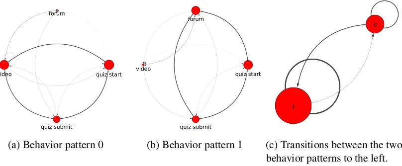
(a) Behavior pattern 0 (b) Behavior pattern 1 (c) Transitions between the two behavior patterns to the left.

Figure 1: An idealized example of what our behavior representation could capture.

How should we represent behavioral patterns, and what does it mean to understand changes in student behavior with respect to these patterns? These are still very open questions and are active areas of research (Kizilcec et al., 2013; Faucon et al., 2016; Davis et al., 2016; Shih et al., 2010). In this paper, we advocate for a representation of student behavior patterns as well asbehavior transitionsthat we believe is simultaneously interpretable but also amenable to unsupervised, automated discovery via statistical means. Specifically, we choose to visualize behavior patterns as labeled directed graphs where a node represents a “behavior state” (such as watching a lecture video or visiting a forum), a directed edge indicates a transition from one behavior state to another, node sizes are proportional to steady-state probabilities, and edge widths are proportional to the probability of leaving a node following that edge. We can use this same representation for visualizing both the student behavior patterns as well as the transitioning behavior between them. In Figure 1 we show a hypothetical example of the kind of output our proposed representation could convey. Here we see two different behavioral patterns (1a and 1b) as well as thetransition behaviorbetween these two behavior patterns (1c). Such a visualized state-transition representation is very informative for describing student behavior. Indeed, we could infer many things from even such a simple example: The first might be that, when students are taking quizzes, they tend to either use the forum or the videos for support, but not both. They also tend to take quizzes in a sort of “cycle” pattern, indicating perhaps that this course allows quiz re-takes. Finally, in Figure 1c we could conclude that users tend to change their quiz-taking behavior over time from one that is more video-focused (pattern 0) to one that is more forum-focused (pattern 1).

Our proposed model (as well as the proposed behavior representation) is motivated by the following observations:

1. Student behavior is complicated and cannot necessarily be captured sufficiently by rule-based methods such as those explored by Kizilcec et al. (2013) and Davis et al. (2016). We instead propose to treat student behavior patterns as being characterized (represented) via a sequence oflatent states. This allows us to automatically capture patterns that we might not have been able to articulate clearly a priori via a series of rules, and allows us to model the inherent uncertainty in assigning a student’s behavior to a pattern or group.

2. Student behavior can vary over time. Previous models that treat students as exhibiting only one behavioral pattern over time (Faucon et al., 2016) miss out on the opportunity to understand student behavior dynamics in a course. We propose a latent space model with

latent state transitionsto flexibly model the dynamics.

3. Analysis of student behavior can and should be performed at varying levels of granularity. This requires us to aggregate data over time withdifferent levels of resolution; existing models tend to come with an assumption about the resolution of time they consider (Faucon et al., 2016; Kizilcec et al., 2013; Shih et al., 2010). We propose a model that is agnostic to the time resolution considered, allowing it to be applied at different levels of resolution more naturally.

Thus, what we propose is alatent variable approachfor mining student behavior patterns that isprobabilisticfor inference and doesnotforce assumptions about time resolutions, making itflexible to model state changes over different time resolutionsmore easily. More specifically, we propose a novel two-layer hidden Markov model (2L-HMM) to discover latent student behavior patterns via unsupervised learning on large collections of student behavior observation sequences. Evaluation results on a MOOC data set on Coursera demonstrate that the 2L-HMM can effectively discover a variety of interesting interpretable student behavior patterns at different levels of resolution, many of which are beyond what existing approaches can discover. We show that the patterns uncovered by the 2L-HMM capture meaningful behavior by quantitatively showing that features extracted from a trained 2L-HMM correlate with learning outcomes. Since our proposed methods are unsupervised, they can potentially be applied to any MOOC data without requiring manual annotation effort at the level of sequences, thus empowering instructors to use the latent patterns discovered by the 2L-HMM to further extract knowledge about the behaviors his/her students exhibit in the MOOC.

2. R

W

Our model is based heavily on the prior art of Hidden Markov Models (HMMs) (Rabiner, 1990) for sequence labeling tasks. As a member of the more general family of probabilistic graphical models (Koller and Friedman, 2009), HMMs are widely applicable and have been used for tasks such as speech recognition (Huang et al., 1990), part-of-speech tagging (Jurafsky and Martin, 2009), and econometrics (Hamilton, 1990). A major challenge in applying HMMs and other graphical models successfully to solve a problem is to design an appropriate architecture of the model, which always varies according to specific applications.

the part-of-speech category for a word. In speech recognition (Huang et al., 1990), the output distributions might be mixtures of Gaussians to predict real-valued vectors extracted from short windows of a speech signal. In the domain of econometrics, Hamilton (1990) explores HMMs in the context of “regime-switching.” In this framing, the goal is to understand how econometric data changes by modeling discrete changes in “regime” as having an impact on the resulting real-valued vector data observed. The “regimes” are thus represented with a model that can produce real-valued vector data, such as a multivariate Gaussian or an auto-regressive model. The analogy with HMMs is that a “regime” is a latent state, and the characterization of the regime itself is the output distribution for that latent state. Our model can be seen as such a “regime-switching” model where the output of the “regimes” that students are switching between are discrete-valuedsequences(as opposed to real numbers, vectors of real numbers, or categorical symbols) and the model used to represent a specific “regime” is an (observable) Markov chain over the observed student actions. We view the switching between “regimes” as the first “layer” of our model, and the transitioning behaviorwithina “regime” between the actions a student takes as the second “layer” of our model.

A multi-layered approach to HMM modeling of sequence data has been performed before in other domains. Zhang et al. (2004), for example, explored a two-layer HMM framework for modeling actions in meetings, but their definition of “two-layer” differs from ours. In their formulation, the “lower-layer” level is used to label audio-video action sequences into basic events, and the “upper-layer” is used to label the output of the lower-layer to discover higher-level office behavior abstractions. Oliver et al. (2004) propose a similar layered HMM approach for modeling office activity at multiple different levels of time granularity. In their approach, each layerLis represented as a “bank” ofKdifferent HMMs that model sequences of some length TL. At the bottom layer (L = 1), the bank ofK HMMs corresponding to that layer is run on

some initial observation data, considering windows of observations of lengthT1. Then an output

is generated by using the inferential results of theseK HMMs to make a prediction: which of the K HMMs was most likely to produce that sequence of observations? This output is then fed to

the next layer of HMMs, which considers sequences of lengthT2 and outputs prediction results

as to which of theK HMMs at layer two were most likely to produce the sequence of outputs

produced by the previous layer, and so on.

Our formulation differs from both Zhang et al. (2004) and Oliver et al. (2004) in that we do not feed the labeled sequence of the lower level into the input of the higher level. Instead, our lower level is treated using a non-hidden Markov model, and the higher level is modeling transitions between theK different non-hidden Markov models we consider. The problem to

be solved is similar in that we wish to predict a “label” for a sequence of actions a student takes as well as understand the transition behavior between those labels. However, one of the consequences of modeling the lower layer using a non-hidden Markov model instead of an HMM directly is that the meaning of the K different latent states can be more clearly captured by

By taking a more restrictive view of the first layer, we can produce a representation that can be more readily interpreted due to the states in our first layer representation having an immediately clear meaning (the concrete action they represent).

The 2L-HMM model we propose is more closely related to the Hierarchical Hidden Markov Model (HHMM) detailed in Fine et al. (1998). Here, the “layers” are modeled by having the hidden Markov model have two kinds of transitions. Horizontal transitions move between states within a layer, where vertical transitions move between different layers. At the bottom layer lie the “production” states, which output symbols according to some probability distribution. Our specific model, in this case, can be modeled as an HHMM where the horizontal transitions between nodes at the highest layer (including self-loops) mustbe immediately followed by a vertical transition to the lower layer. The output probability distributions over symbols in the lower layer “production” level are forced to emit only one kind of symbol, and vertical transitions are only allowed into the original higher-layer state that transitioned down into the lower-layer.

Mixtures of hidden Markov models are also conceptually similar to our formulation. Song et al. (2009) explored using a mixture of hidden Markov models in the context of anomaly detection in the security domain. Ypma and Heskes (2002) use mixtures of HMMs to categorize web pages and cluster users by investigating web log data, which is quite similar to the clickstream log data we obtain from MOOCs. The major difference between our approach and a standard mixture of HMMs is that we also model thetransition behaviorbetween the Markov models that make up our model’s lowest layer, where a standard mixture of HMMs would ignore the potential dependence of the previous sequence’s latent state on the next sequence’s latent state.

HMMs or similar ideas have been previously applied to model education data (Shih et al., 2010; Kizilcec et al., 2013; Davis et al., 2016), but the previous models are not well tuned toward the student behavior task and thus cannot adequately address all the aspects of the complexity of student learning behavior. A main technical contribution of this paper is to propose a more general HMM that can better adapt to the variations of student behavior via its variable resolution and nested HMM structure, and thus enable discovery of more sophisticated behavior patterns and provide a more detailed characterization of student behavior than the previous models.

For example, Kizilcec et al. (2013) assigned students to states following a rule-based approach based upon when the student submitted the assignment for a particular week in the course. They investigated how students transitioned between these states as the course progressed, and used the sequence of states a student exhibited as a representation for performingk-means clustering

of students into related groups. This differs from our method substantially: we assign students to states using a probabilistic framework to account for uncertainty in this state assignment and jointly learnrepresentations for these states, which are treated as being latent as opposed to pre-defined using some rule (or set of rules). Furthermore, our model provides more flexibility in how the time segments are defined, allowing for both finer (for example, day-by-day) or coarser (for example, month-by-month) granularity. Shih et al. (2010) investigated the use of HMM-based clustering techniques for automatic discovery of student learning strategies when solving a problem. This is similar to our approach in that the description of behavior profiles is a Markov model, but cannot further characterize each latent state with another informative HMM. Thus, their work can be regarded to modeling “micro” behavior, whereas our model can model both “micro” and “macro” behavior.

by an automatic (rule-based) assignment of all sequences to these motifs. Our method, by contrast, attempts to do this automatically: the latent state representations obtained by our model attempt to capture similar meanings to their behavior motifs in a completely automated fashion. They also automatically generate and investigate Markov models for different MOOCs, but do so by consideringallstudent action sequences as belonging to asingle Markov model. In our approach, we allow each student behavior sequence to belong to one ofK different Markov models (and

further model the transition probabilities between these latent state Markov models between each sequence a student generates). Thus, their Markov models presented are a special case of our model whenK = 1.

Faucon et al. (2016) proposed a semi-Markov model for simulating MOOC students. They produce behavior profiles that characterize groups of students in the form of semi-Markov models like our proposed model does, but they assume that a student can belong to only one behavior profile across the entire course rather than allowing this profile to change over time. Because we do not have this restriction, our model is also able to learn the transition probabilities between the different behavior profiles we discover.

There are a few additional related studies worth mentioning. Bayesian Knowledge Trac-ing (Corbett and Anderson, 1994) in its basic form uses a hidden Markov model to model the probability that a learner knows a certain skill at a given time. Modifications to this algorithm include contextual estimation of the “slip” and “guess” probabilities of the model (Baker et al., 2008) and most recently a re-framing as a neural network problem (Piech et al., 2015).

3. A T

-L

HMM

MOOC L

A

Our general idea is to use a probabilistic generative model to model the student activities as recorded in a MOOC log, which means we will assume that all the observed student activities are samples drawn (i.e., “generated”) from a parameterized probabilistic model. We can then estimate the parameter values of the probabilistic model by fitting the model to a specific MOOC log data set. The estimated parameter values could then be treated as the latent “knowledge” discovered from the data. Because such a generative model attempts to fitallthe data, it enables us to discover interesting patterns that can explain theoverallbehavior of a student or thecommon

behavior patterns shared by many students.

An HMM is a specific probabilistic generative model with a “built-in” state transition system that would control the data to be generated by the model, thus it is especially suitable for modeling sequence data (Rabiner, 1990; Huang et al., 1990). At any moment, the HMM would be in one ofkstatesU ={u1, . . . , uk}, and at the next moment, the HMM would move to another state

stochastically according to a transition matrix that specifies the probabilityp(ui |uj)of going

to stateui when the HMM is currently in stateuj. When the HMM is in stateu, the HMM can

generate an observable data pointxaccording to an output probabilistic modelp(x|u). Thus,

if we “run” an HMM forN time points denoted byt = 1, . . . , N, the HMM could “generate”

a sequence of observationsx1. . . xN, where each xi is an output symbol by going through a

sequence ofhidden statesw1. . . wN where eachwi is a random variable taking a value from

the HMM’s state setU. The association of such a latent sequence of state transitions with the

student behavior more deeply than a model with no latent state variables.

In many ways, the generation process behind an HMM is meant to simulate the actual behavior of a student. We may say that students transition through different “task states” (or “behavior states”) in the process of study. One such task state may be to learn about a topic by mostly watching lecture videos, another task state may be to work on quizzes, and yet another may be to participate in forum discussions. While in each of these different states, the student would tend to exhibit different surface “micro” behaviors. For example, in the lecture study state, the student would tend to have many video-watching related behaviors and occasionally forum activities, while in the quiz-taking state (to pass each module), the student would tend to show many quiz-related “micro” activities as well as asking questions or checking discussions on the forum. Note that due to the complexity of the student behavior, it is very difficult to accurately

prescribe the specific surface “micro” behavior patterns for each state in advance, especially without prior knowledge about the students. For example, forum activities are likely interleaved with other activities in every task state and the interleaving pattern can be somewhat irregular with potentially many variations. The major motivations for using an HMM are that (1) it uses a probabilistic model (the output probability distributionp(x_|u)conditioned on each state) to

directly capture the inevitable uncertainty in the association of surface “micro” activities with their corresponding latent task/behavior state, which is often our main target to discover and characterize, and (2) it does not make any assumption about which latent task/behavior state must be associated with which observed activities or how a student would move from one state to another, but instead allows our data to “tell” us what kind of associations are most likely, what kind of transitions are most probable, and which states tend to be more long-lasting for any set of students.

However, if we were to use an ordinary HMM to analyze our data, we would treat each observed “micro” activity (such as video watching or forum post reading) as an output symbol, and thus the output distribution p(x | u) for each discovered latent state would be a simple

distribution over all kinds of observable micro activities recorded in our log data (e.g., 50% lecture watching, 8% quiz taking, 7% quiz submission, 2% course wiki reading, etc.). While such a distribution is meaningful and can already help us interpret the corresponding latent state, it only gives us a rather superficial characterization of student behavior.

Ideally, we wantp(x_|u)to characterize the directly observable “micro” behavior in more

detail to further capture the relations and dependencies of these “micro” activities. To this end, we would treat an entire sequenceof “micro” activities (e.g., one session of activities) as an observed “symbol” from a latent state, and further model the generation of such a sequence with another Markov model where we treat each micro activity as anobservablestate, and model the transitions between these activity states in very much the same way as the state transitions in an HMM.

To estimate the parameters of our model, we will use the EM algorithm (Dempster et al., 1977) which allows us to perform maximum likelihood estimation of the model in the presence of latent (unobserved) variables. This algorithm, intuitively, works as follows: first, the model parameters we wish to estimate are initialized to some random (but valid) starting point. Then, we “guess” what the latent variable values might be given the current model parameters. We can then use this guess to re-estimate the model parameters, which will improve their accuracy slightly. We can then use these newly estimated parameters to again “guess” what the latent variable values might be, and so on. We repeat this process until the parameter estimates no longer shift by much (or, equivalently, the log likelihood of the data does not improve by much). The computation for the “guessing” of latent variable values is somewhat involved in the case of HMMs (see Section 3.3. for the full details), but the general intuition behind the iterative hill-climbing remains valid.

Next, we present this model more formally and discuss how to estimate its parameters to uncover these latent patterns in an unsupervised manner.

3.2. FORMALDEFINITION OF THE 2L-HMM

Given a MOOC log, we can define a setAof actions that a student can take at any given time.

For example, an actiona _∈A might be “viewing lecture,” “taking quiz,” or “viewing forum.”

For each student in the course` ∈ L, we then extract a list of action sequencesO` that he or

she produced as observed in the log, where each sequence o _∈ O` is itself a list of actions (a1, a2, . . . , aT)with eachai ∈A. Each sequence can be divided flexibly; in this paper, we chose

to denote the end of a sequence as occurring when no further actions occur within a 10-hour window of time (and thus our sequences roughly correspond to one day’s worth of activity). This decision reflects our desire to uncover latent state transition behavior at the granularity of day-to-day behavior. A different segmentation strategy could be used to uncover hour-by-hour behavior or week-by-week behavior, and this depends entirely on the desired time resolution one wishes to be exhibited in the transitions between the latent states. Different segmentation strategies will result in different underlying training data, and thus different meanings behind the patterns that the 2L-HMM will extract. The flexibility of using different segmentation strategies is intentional as it allows a user to adjust the segmentation as needed to obtain patterns at different granularity levels.

Each sequenceo_∈O`is associated with a latent stateu∈ {1, . . . , K}(whereK is a fixed

constant picked in advance). The actions within the sequence o = (a1, a2, . . . , aT)are then

modeled as a first-order Markov process conditioned uponuwhere each action is drawn from

a distribution conditioned upon the previous action (except for the first which is sampled from an initial starting distribution). We can write the parameters for the first-order Markov model associated with latent stateuas λ(u) _{= (π}(u)_{, A}(u)_)whereπ(u) _{indicates the initial probability}

vector of length|A_|andA(u)_{is an|A|×|A|matrix indicating the transition probabilities between}

each pair of actions fromA.

Thus, the probability of a sequenceoof lengthT given a latent stateuis

P(o|λ(u)) =P(a1 |π(u)) T Y

i=2

P(ai |ai−1, A(u)) (1)

whereP(a | π(u)_{) = π}(u)

A(aui−)1,ai is the transition probability of moving from actionai−1 to ai given that the model is currently in latent stateu.

We can compute the likelihood of a list of action sequencesO` of lengthN for a student`by

marginalizing over all possible latent state sequences(v1, . . . , vN)∈U as

P(O` |Λ) =

X

(v1,...,vN)∈U

P(v1 |Λ)P(o1 |λ(v1))×

N Y

i=2

P(vi |vi−1,Λ)P(oi |λ(vi)) !

(2)

whereΛis the set of all model parameters. In our model, we letΛ = (π, A, B)whereπandA

are the parameters of a first-order Markov model over the latent states andB = (λ(1)_{, . . . , λ}(K)₎

where eachλ(i)_{consists of the parameters for the first-order Markov model over action sequences}

for latent statei. Thusπ(without superscripts) is an initial probability vector of lengthK and A(without superscripts) is aK ×K transition probability matrix, analogous to the case with

the individual first-order Markov model parametersλ(i)_{for each latent state. We have in total} K+K2_+K(|A|+|A|2_{)parameters to be estimated from our sequence data.}

This can be seen as a modification of the traditional hidden Markov model with categorical outputs (Rabiner, 1990) where instead of discrete observations (one for each latent state tran-sition) we have observations that take the form of entire sequencesoi = (a1, a2, . . . aT)whose

probabilities are computed using another (non-hidden) Markov model conditioned upon the latent stateui.

3.3. PARAMETER ESTIMATION

To learn the parameters of our model, we may use maximum likelihood estimation. Unfortunately, a closed-form solution does not exist, so we must appeal to the EM algorithm (Dempster et al., 1977). In particular, we propose a minor modification of the Baum-Welch algorithm (Rabiner, 1990) which is an efficient EM algorithm for learning the parameters of hidden Markov models in an unsupervised setting where the Markovian assumption is exploited to significantly reduce the computational complexity of the EM algorithm by avoiding explicit enumeration of all the possible state transitions. In the following sections, we will provide a brief description of the original Baum-Welch algorithm for unsupervised parameter estimation for categorical valued hidden Markov models, and then describe our modification to allow for parameter estimation for our 2L-HMM modification for sequence valued observations.

3.3.1. Baum-Welch for Traditional HMMs

In the traditional HMM formulation with categorical outputs, we haveΛ = (π, A, B)whereπ

is the initial probability distribution over the latent states (of lengthK),Ais aK _×K matrix

indicating the latent state transition probabilities, and B = (b1, . . . , bk)is a length K vector

where each entrybiis a probability distribution over the possible discrete output symbols fromA.

The goal of the Baum-Welch algorithm (also called the forward-backward algorithm) is to learn the values for the parameters Λ from a collection of observed sequences of values

fromA. Concretely, our training dataD = (o(1)_{, . . . ,o}(M)_{) is a collection of M sequences}

o(k)_{, each of which consists ofT}

ksymbols (observations) fromA. The Baum-Welch algorithm

defines two sets of variablesα(to)(i)called the forward variables andβ

(o)

t (i)called the backward

α_t(o)(i) = P(o1, . . . , ot, vt =i|Λ)is the probability of generating the sequence of

observa-tions(o1, o2, . . . , ot)up to timetand arriving in stateiat that time. They are typically defined

using the following recursion:

• α(₁o)(i) = πibi(o1), the probability of starting in state i (πi) times the probability of

generating the first observationo1 from statei.

• α(_to₊₁)(i) = bi(ot+1)PK_j=1α(to)(j)Aji, the probability of generating the observation ot+1

from stateitimes the probability that we arrive in stateifrom any other previous state after

generating all of the other observations.

Analogously,β_t(o)(i) = P(ot+1, . . . , oT |vt=i,Λ)is the probability of generating therest of

the sequencegiven that we are in stateiat timet. They are also defined using a recursion:

• β_T(o)(i) = 1

• βt(o)(i) = PK

j=1β (o)

t+1(j)Aijbj(ot+1), the probability of transitioning to any state j and

generating the observationot+1 times the probability of generating the rest of the sequence

given that we transitioned to statej.

Given theαs and theβs, we can computeγ_t(o)(i), the posterior probability of being in a given

stateiat timet, andξt(o)(i, j), the posterior probability of going through a transition from statei

to statejat timetas

γ_t(o)(i) = α

(o)

t (i)β

(o)

t (i) PK

j=1α (o)

t (j)β

(o)

t (j)

(3)

and

ξ_t(o)(i, j) = α

(o)

t (i)Aijbj(ot+1)βt(+1o)(j)

PK j=1α

(o)

t (j)β

(o)

t (j)

(4)

respectively (Rabiner, 1990). Computing these variables for each sequenceo_∈Dis the E-step

of the EM algorithm.

Givenγ_t(o)(i)andξ_t(o)(i, j)for each sequenceo_∈D, we can update our model parametersΛ

as

πi = P

o∈Dγ

(o)

1 (i)

|D_| , (5)

Aij = P

o∈D

PT t=1ξ

(o)

t (i, j) P

o∈D

PN j=1

PT t=1ξ

(o)

t (i, j)

, and (6)

bi(a) = P

o∈D

PT

t=1,ot=aγ

(o)

t (i) P

o∈D

PT t=1γ

(o)

t (i)

(7)

3.3.2. Baum-Welch for HMMs with Sequence Observations

The major deviation of our model from the traditional categorical-valued HMM is that our observations are themselves sequences of actions fromA rather than individual tokens. We

again denote our parameters as Λ = (π, A, B) whereπ is the initial probability distribution

over the latent states (of lengthK),Ais a K×K matrix indicating the latent state transition

probabilities, but B = (λ(1)_{, . . . , λ}(K)_{)is now a vector of length K where each elementλ}(i)

consists of the parameters for a first-order Markov model over the action spaceA. Recall that

eachλ(i) _{= (π}(i)_{, A}(i)_)whereπ(i)_{is an initial action distribution over the|A|available actions,}

andA(i)_{is the|A| × |A|transition matrix between those actions.}

The goal of the Baum-Welch algorithm is still to learn the parametersΛfor our model. What

differs from the categorical-valued HMM case is that our data now consists of a collection oflists

of sequences, rather than just a collection of sequences. This means that our observation values

otare nowthemselvessequences of values fromA, rather than just being a single token from

A. Formally, our training dataD = (O(1)_{, . . . ,O}(|L|)_{), where eachO}(`)_{= (o1, . . . ,o}

T`)is itself a list of sequences. Each sequenceok∈O(`)consists of a list of actions(a1, . . . , aTk), each of which is a member ofA.

In order to run the forward-backward algorithm for an elementO∈Dto compute theαand βrecursions like before, we must definebi(ot)in this setting whereot = (a1, . . . , aTt)is now a sequence instead of a single token. We define it as follows:

bi(ot) =P(ot|λ(i)) =P(a1 |π(i)) Tt

Y

k=2

P(ak |ak−1, A(i)) =πa(i1)

Tt

Y

k=2

A(_ai_k)_−1,ak. (8)

Fortunately, the recursions for α(_tO)(i) and β_t(O)(i) remain the same, as do the definitions of

γ_t(O)(i)andξ_t(O)(i, j), in the E-step. We can simply substitute the new definition for the output

distributionbi(ot)in those equations.

The substantial change is in the updating equations in the M-step, where we replace the update forbi(a)(which used to be a categorical distribution) by a pair of updates for the Markov

chain for statei: one forπa(i)one forA(_abi). The two updates can be written as

π_a(i) = P

O∈D

P

ot∈O,ot,1=aγ

(O)

t (i) P

O∈D

P

ot∈Oγ

(O)

t (i)

, and (9)

A(_abi) = P

O∈D

P

ot∈O

P|ot|

m=2,ot,m−1=a∧ot,m=bγ

(O)

t (i) P

O∈D

P

ot∈O

P|ot|

m=2,ot,m−1=aγ

(O)

t (i)

. (10)

These updates can be understood as follows. π(ai)is the probability that a sequence being generated

by stateibegins with actiona. γ_t(O)(i)gives the probability of generating the sequenceotfrom

statei, so we simply aggregate this for all sequences ot where the first action isa. We then

normalize this distribution to sum to 1 across all possible actions a ∈ A to obtain our new

estimate forπ(ai). A(_abi)is the probability that a sequence being generated by stateicurrently at

actiona ∈ A transitions to action b ∈ A. Thus, we compute the expected number of times

we observe a transition from ato bin a sequence generated by statei, and we normalize this

distribution to sum to 1 across all possible actions b _∈ A. Our modified EM algorithm for

Table 1: Statistics about the sequences extracted from the two MOOCs.

MOOC Students Sequences Avg. |s|

textretrieval-001 18,941 85,240 7.31 sustain-001 85,240 231,881 15.4

4. E

R

As an analysis tool, the 2L-HMM model provides us with the following two patterns to character-ize student behavior: (1) the latent state representations, and (2) the latent state transitions. Thus, to evaluate the proposed model, we conduct experiments to qualitatively analyze both types of patterns discovered from empirical MOOC log data.

Specifically, we look at the MOOC logs associated with two different Coursera MOOCs offered by UIUC: textretrieval-001 and sustain-001. The textretrieval-001 MOOC represents a highly technical computer science course, where the sustain-001 MOOC is more representative of a humanities course. We picked these two MOOCs because of their vastly different content domains. Table 1 summarizes the two datasets we extracted from the MOOCs.

4.1. LATENTSTATE REPRESENTATIONS

The 2L-HMM is meant to be a tool for exploratory analysis of student behavior. As such, the number of states should be empirically set based on the goal of analysis. A higher number of states will lead to a finer-grained modeling of student behavior. In our experiments, we explored using between 2–6 states. First, we fit a 6-state 2L-HMM to the textretrieval-001 sequence dataset and show some of the latent state representations we find. We used the following ten actions as our action set A: (1) quiz start, (2) quiz submit, (3) wiki (course material), (4) forum list

(view the list of all forums), (5) forum thread list (view the list of all threads in a specific forum), (6) forum thread view (view the list of posts within a specific thread), (7) forum search (a search query issued against the forum), (8) forum post thread (a new thread was posted), (9) forum post reply (a new post was created within an existing thread), and (10) view lecture (defined as either streaming or downloading a lecture video).

To visualize these Markov models that represent our latent states, we plot them as a directed graph where we set the size of a node to be proportional to its personalized Pagerank score (Page et al., 1999; Jeh and Widom, 2003) where the personalization vector is the initial state distribution for the Markov model. We let the thickness of a directed edge(u, v)reflect the probability of

taking that edge given that a random walk is currently at noteu(as indicated by the transition

matrix)1_{. In the interest of reproducibility, the source code for analyzing the MOOC logs we}

use in this paper and for producing the figures themselves is publicly available as open-source software2_.

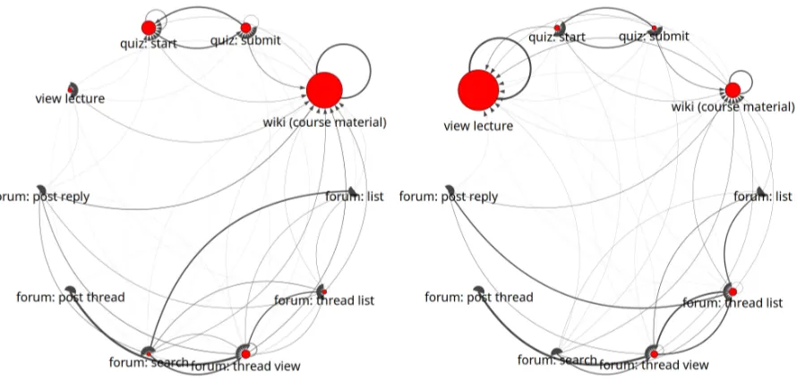
Figure 2 includes two such representations we learned. Under our interpretation, the first corresponds to a “quiz taking” state (it has higher “quiz: start” and “quiz: submit” state

probabili-1_{We do not plot the transition probabilities directly within the figure to ease readability; we instead will mention} relevant transition probabilities in the text as we discuss the plots. The plots were created using python-igraph:

http://igraph.org/python/.

(a) An example “quiz taking” state. (b) An example “lecture viewing” state.

Figure 2: Two example states found by the 6-state 2L-HMM. (The naming of these states reflects our own interpretation.)

ties than the other five states) whereas the second corresponds to a “lecture viewing” state. Our unsupervised method can uncover states that do indeed correspond to student behavior modes that we would expect to find a priori.

We also argue that it is important that the latent state representation is a Markov model rather than just a discrete distribution over actions inA(as would be the case for a traditional

single-layer HMM). We can observe why if we take a closer look at each of the two latent state representations in Figure 2 and look at their forum component (bottom right). We can see that the relative probability of the forum activities is roughly the same between these states, but the

transitionsare quite different. In Figure 2a we have a relatively low probability of walking from the “forum thread view” action back to the “forum thread list” action (see the bottom rightmost arc; transition probabilityp_≈0.17), but in Figure 2b we actually observe a much stronger link in

this direction (transition probabilityp≈0.63). This difference highlights an important distinction

between these two latent states: in the first you are more likely to visit the forumlooking for a post, where in the second you are more likely to visit the forumto browse existing posts. Thus, capturing the action transition matrix within a latent state is important for capturing detailed insights involving bigrams of actions.

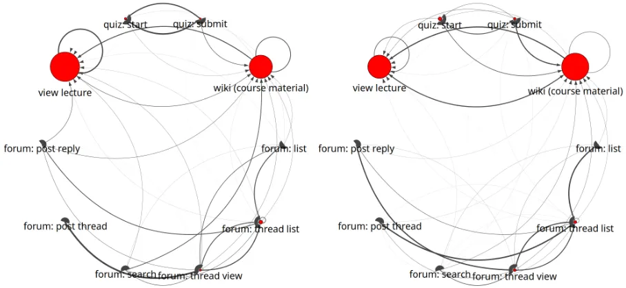
We can also use our model for cross-course behavior analysis. In Figure 3 we show two latent state representations learned by a 6-state 2L-HMM, one from textretrieval-001 and one from sustain-001. These two states were chosen as they are the most similar between the two courses. However, if we look at the transitions we can see some important differences. First, in the state from textretrieval-001, we can see that the probability of returning to the course wiki after viewing a lecture (transition probability p ≈ 0.24) is considerably lower than that

(a) A state from textretrieval-001. (b) A state from sustain-001.

Figure 3: Two similar example states found by the 6-state 2L-HMM.

the self-loop for staying in a lecture activity in textretrieval-001 (transition probabilityp_≈0.70)

is significantly higher probability than it is in the state from sustain-001 (transition probability

p_≈0.34). This gives us some insight into the lecture viewing behavior of students in these two

MOOCs which might reflect the course’s structure (which, as demonstrated in Davis et al. (2016), can differ substantially across different MOOCs). In textretrieval-001, students are likely to view lecture videos in succession directly without first visiting the course wiki, whereas in sustain-001 students are much more likely to first return the course wiki before watching the next lecture video. This observation would be lost if we did not consider the transitions between the actions within the latent states.

4.2. VARYING THE NUMBER OF LATENT STATES

Our 2L-HMM model has a parameterKthat sets the number of latent states to be learned. We

believe that this can allow our model to flexibly discover patterns of different granularity, and we can show this by varyingKfor a course and observing how the latent state representations

evolve.

In Figure 4 we see3_{the evolution of the latent state representations found for the}

textretrieval-001 MOOC. WithK = 2we uncover a video watching pattern (state 1) and a course material

browsing pattern (state 0). However, we can see that whenK = 3we can uncover a new pattern

involving forum behavior in state 3 (notice the node sizes on the bottom right). As we increaseK

to four, we can see that state 1 splits into state 1 and state 3. These states appear quite similar at a glance, but there are still some key differences. First, we can see that state 1 now has a non-negligible forum component, whereas state 3 has hardly any weight on the forum.

We observe similar behavior in Figure 5 as we increaseK when fitting our 2L-HMM on the

State

0

(W

iki)

State

1

(Lectur

e)

State

2

(Thr

ead

V

iew)

State

3

(Lectur

e/W

iki)

Figure

4:

The

ev

olution

of

states

for

increasing

K

for

the

te

xtretrie

val-001

MOOC.

Each

ro

w

corresponds

to

the

ne

xt

value

of

K

,starting

from

K

=

2

.State

“names”

indicate

the

highest

probability

action(s)

within

the

State

0

(W

iki)

State

1

(Lectur

e/W

iki)

State

2

(Thr

ead

List)

State

3

(Thr

ead

V

iew)

Figure

5:

The

ev

olution

of

states

for

increasing

K

for

the

sustain-001

MOOC.

Each

ro

w

corresponds

to

the

ne

xt

value

of

K

,starting

from

K

=

2

.State

“names”

indicate

the

highest

probability

action(s)

within

a

(a) (b) (c)

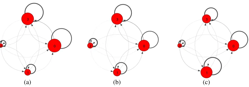
Figure 6: The latent state transition diagrams for a 4-state 2L-HMM fit to textretrieval-001 for all students (a) compared to only “perfect” students (b) and only “low” students (c).

sustain-001 MOOC. Again, in the transition betweenK = 2and K = 3, we discover forum

behavior patterns as a latent state. However, in the transition betweenK = 3 toK = 4, we

instead see a refining of that discovered forum state, where state 3 captures asymmetric transition probabilities between “forum thread view” and “forum thread list”. These states could be seen as redundant, in which case a setting ofK = 3may be more appropriate for the sustain-001 dataset.

4.3. TRANSITIONSBETWEEN LATENTSTATES

A unique property of our model is its ability to capture transitions between thebehavior patterns themselvesthat are captured by the latent states. In Figure 6a we show the latent state transition diagram for a 4-state 2L-HMM fit on textretrieval-001. We can immediately observe two things: (1) each latent state has a very high “staying” probability, and (2) the prevalence of each latent state matches our intuition. In particular, we can see that the forum browsing state (state 2) has relatively lower probability than the other states as we might expect. It also makes sense that state 0 has a rather high probability as this state likely captures all sequences where a student logged in to the platform and then did nothing else (likely checking for updates). If we look at state 1 and state 3, their relative probabilities match our intuition as well. State 1 seems to capture a more engaged browsing session, where there is non-negligible probability associated with different activities such as quiz taking and forum browsing and, importantly, these activities have high probability symmetric edges (so students are taking quizzes one after the other, or viewing forum threads in succession). By contrast, state 3 seems to capture a more passive student, with negligible probability mass associated with forum activity (with low symmetry in the edges). The link between “quiz submit” and “quiz start” (indicating quiz repetition) is also significantly lower than state 1.

Table 2: Average rank for “perfect” and “low” student groups in the ranked lists associated with the four latent states found by a 2L-HMM. †indicates statistically significant different mean

ranks atp <0.01according to an unpairedt-test.

Group State 0 State 1† _{State 2}† _{State 3 State 2→2}†

Perfect 975.3 1001.5 999.0 1056.5 939.6

Low 1024.9 816.4 1230.5 1161.2 1187.4

decreased. State 1 had its probability increase, but only very slightly.

In Figure 6c we plot the latent state transition diagram for a second group of “low” students. These students were selected so that they attempted all required quizzes in the course, but such that their average quiz score was ≤ 70%. Here, we see that state 1 has a large increase in

size, where we might have expected state 3 to grow instead. However, there is an alternative explanation for this phenomenon. Since state 1 seems to indicate a highly engaged student, it is a perfectly reasonable explanation for the “low” student group as they are going to be working hard to try to fill in the gaps in their knowledge. By contrast, the “perfect” student group likely has many members who can take the quiz more passively and get perfect marks, perhaps because they already know much of the material being presented, or are just naturally strong and do not require much background review to perform well. This also explains why state 1 did not increase in size for the “perfect” group like we were anticipating. Kizilcec et al. (2017) observe similar phenomena with the courses they studied where they find that certificate earning is negatively correlated with help seeking behavior. Our model lends itself well to discovering this potentially counter-intuitive insight directly from data.

To quantify this finding, we perform the following experiment. First, we select all students from textretrieval-001 who completed all of the quizzesLq ⊂L. This gives us 1,985 students

along with their average quiz score. We then create a ranked list of the students inLqby sorting

them by their “preference” for a specific latent state

p`(i) =

PT t=1γ

(o`)

t (i) PK

j=1

PT t=1γ

(o`)

t (j)

(11)

whereo` is the list of action sequences for student` andγ is defined as before and computed

using the Baum-Welch algorithm. We can now compare the average rank in this list for both the “perfect” student group and the “low” student group: a useful state for distinguishing the two groups should result in a ranked list with statistically significant differences in average rank between the two groups. Our results are summarized in Table 2. Indeed, we discover that states 1 and 2 are correlated with the “perfect” or “low” groups: state 1 ranks students in the “low” group significantly higher than those in the “perfect” group, and state 2 does the opposite and prefers students in the “perfect” group to those in the “low” group.

Returning to Figure 6, we can also see a difference in the transitions between the latent states. In particular, look at the transitions in Figure 6b and Figure 6c that leave state 2. In the “perfect” group, nearly all this probability mass is allocated for the self-loop (p ≈ 0.93). In the “low”

group, this self-loop is less strong (p_≈0.80; most easily seen by noting that the edges leaving

given that a student`is already in state 2, how likely are they to remain there in the next action

sequence?). This can be computed as

p`(2,2) =

PT−1

t=1 ξ (o`)

t (2,2) PK

i=1

PT₋1

t=1 ξ (o`)

t (2, i)

(12)

whereξis defined as before and computed using the Baum-Welch algorithm. The last column

of Table 2 indicates that this transition feature also correlates with the achievement group and results in significant differences in mean rank.

5. L

P

D

There are a few limitations of our model that are important to highlight. First, there are specific technical limitations due to the statistical nature of the model and the particular methodology we propose for fitting our model parameters. Second, there are limitations in the kinds of patterns our model is able to discover in its current formulation and the ease with which instructors are able to extract knowledge from these patterns. We discuss both lines below.

5.1. TECHNICALLIMITATIONS AND IMPLEMENTATION CHALLENGES

One potential limitation is that the model is complex and has many parameters in order to truly uncover the relevant patterns in the data. To properly estimate these parameters at training time, a large amount of data must be available to the training algorithm. The assumption that we have a large amount of sequence data available for training on should hold for most MOOC courses, but this assumption may be problematic if attempting to apply our model to smaller online (or on-campus) courses.

Our model fits its parameters using maximum likelihood estimation using the EM algorithm. The EM algorithm is a hill climbing algorithm that is optimizing in a highly non-convex parameter space. Thus, it can only guarantee that we reach a local maximum in practice (Dempster et al., 1977). This may mean that the parameters found for the model may not be the “best” parameters in a global sense, which may lead to suboptimal latent state representations and transition patterns. Empirically, however, we observed in our experiments that strong patterns tend to always show up if algorithm reaches a reasonably good local maximum, and the differences of the results tend to be related to weak “unstable” patterns which may not be reliable anyway. Since it is far more important and useful to reveal the strong salient patterns than weak unreliable ones for instructors, the problem might not necessarily affect the utility of the approach so significantly. A commonly applied approach to address the problem of multiple local maxima is to run the model multiple times with different starting points to allow the model to explore a larger portion of the parameter space. One can then compare the log-likelihood of the data between the models that were started from different initialization points and select the one that has the highest value. This still does not guarantee that we find a global maximum, but it does help alleviate the potential for finding a particularly bad local maximum. In practice, we have found that our model can be fit to the data quickly on commodity hardware, so running it multiple times to address this concern is not computationally unfeasible.

with its length. While there are general approaches to avoiding numerical underflow in hidden Markov models, applying the “scaling” method proposed by Rabiner (1990) will still result in numeric stability issues in our case due to the incredibly small sequence-generation probabilities. We address this in our open-source implementation by computing the trellises in log-space and using the log-sum-exp trick when we need to take summations, which exploits the identity

log n X

i=1

exi _{=a+ log}

n X

i=1

exi−a (13)

whereais typically set tomaxixi to improve stability. We did not encounter further stability

issues once we applied these two tricks.

As is the case with traditional hidden Markov models, it is often important to smooth the underlying model’s distributions to ensure that there is a non-zero probability of generating the observations. We employed a simple additive smoothing in our implementation with a small additive constant (10−6) for all our transition matrices to avoid this problem.

5.2. LIMITATIONS OF DISCOVEREDPATTERNS

The proposed behavior representation is most suitable for representing recurring behavior patterns, which presumably are most interesting to extract from the data, but may not cover all the interesting patterns in the data. It would be interesting to explore other complementary models such as time series models, which may help capture non-recurring patterns.

Our proposed model is flexible in the patterns it can discover in two main ways. The first is that the granularity of the patterns can be adjusted by changing the segmentation strategy one uses to divide the user action stream into discrete “sessions.” The other is the number of latent statesKthat are used to describe the segmented action sequences. One drawback of these two

lines of flexibility is that there is not necessarily a clear answer as to the “correct” approach for both in any given scenario. Varying the segmentation strategy changes the granularity of the patterns the latent states explain, which will change their meaning. Varying the number of latent states increases the flexibility of the model, but also may result in latent states that are not substantially different from the other latent states and/or latent states with very low probability. This flexibility forces a user of our model to make some assumptions about the patterns they wish to find (granularity, diversity), and the model itself does not necessarily provide clear guidance as to what the best approach is.

Furthermore, we have made an implicit assumption that the segmentation strategy is applied as a pre-processing step (and is most obviously a deterministic process). The proposed segmentation strategies in this paper do not specifically allow for the transitioning between the different latent behavior patterns to occur over different windows of time for different users: we have made a strong assumption that transitions between latent states only occur at action sequence boundaries. One can model how much time a user stays in each state in terms of the number of sessions they remain there before transitioning, but it may be better to directly model the amount of time we expect a user to stay in the given state. In other words, a more powerful model might be one in which the segmentation and the latent behavior pattern discovery are jointly modeled in a single probabilistic framework rather than being separate pieces as we investigate in this work.

While the model can discoverpatternsin the data in a fully automated way, there is still clearly a burden on the user of our model to interpret the patterns it has discovered to create actionable

necessary step towards the creation of knowledge, and we view our model as a component in a collaborative system which leverages the machine to perform statistical modeling to extract patterns which then enable a human actor to extract knowledge and take actions on the basis of the data. The pattern discovery is an important and absolutely necessary component, without which it would be very difficult, if not impossible, for humans to directly digest the student behavior buried in the large amount of data. Of course, pattern discovery is only a means to help humans obtain knowledge, not the end of the knowledge discovery process.

6. C

F

W

As a tool to help instructors and education researchers better understand the behavior of MOOC students, we proposed a two-layer hidden Markov model to automatically extract student activity patterns in the form of behavior state-transition graphs from large amounts of MOOC log data. This model is different from existing methods in that it treats behavior patterns as a sequence of

latent states, rather than assigning these states in a rule-based manner. It captures the variable behaviors of students over time and allows analysis at different levels of granularity.

We showed that such a model does, in fact, capture meaningful behavior patterns and produces descriptions of these behavior patterns that are easy to interpret. We argued that it is important to capture student behavior patterns with more sophisticated models than simple discrete distributions over actions to capture information present in bigrams of actions (or larger sequences). By varying the number of latent states inferred, we showed that the model is flexible and can capture patterns of differing levels of specificity in this way. Finally, we investigated whether we can detect differences in student behavior patterns as they correlate with course performance. Specifically, we demonstrated that high-performing students produce substantially different HMM transition diagrams that tend to show longer concentration span in quiz-taking and more active forum participation as compared with the average students. These results show the great potential of the proposed model for serving as a tool to help humans discover knowledge about student behaviors.

There are a number of interesting directions to further extend our work in the future. First, the proposed model is completely general and can thus be easily applied to analyze the log of many other courses to enable deep understanding of student behaviors as well as the correlations of such behaviors and other variables such as grades. To realize these benefits, it would be useful to develop a MOOC log analysis system based on the proposed model to facilitate education research and help instructors improve course design.

Third, there is more recent work on better learning algorithms for mixtures of Markov models (Gupta et al., 2016). It would be worth exploring whether the advances proposed in this and similar work can be applied to our model to address some of the concerns surrounding our use of the EM algorithm for our parameter estimation.

Finally, the proposed model can be extended in several ways. For example, although our model does not explicitly model drop-out like Kizilcec et al. (2013), doing so is an obvious extension. Our model would be able to provide predictions of when a student is “at risk” for dropping out under such an extension. Also, currently, the model learns a transition matrix over the latent states that isshared across all students. It would be interesting to instead learn a different latent state transition matrix for each individual student, but keep the second-level Markov models shared. This would provide the model with more flexibility which may be desirable itself, but would also naturally result in a description of a student (via his or her HMM transitions) that could be incorporated into existing supervised learning techniques that try to predict student outcomes for understanding which of the latent behavior patterns discovered by 2L-HMM are most predictive of the performance of student learning. One could also relax this somewhat and posit thatgroupsof students transition between the lower layer patterns identified by our method in distinct ways; this way, we can do a soft clustering of students intoK2groups

based on the similarity of their transitioning behavior between the higher-level behaviors we can identify.

7. A

The authors would like to thank Hao Zheng, Jason Cho, and Sean Massung for their helpful discussion while developing this work, and the ATLAS group at UIUC for their help with securing the datasets used. We also thank the anonymous peer reviewers whose critical reading and constructive feedback were crucial for improving the final manuscript. This material is based upon work supported by the National Science Foundation Graduate Research Fellowship Program under Grant Number DGE-1144245 and by the National Science Foundation Research Program under Grant Number IIS-1629161.

R

BAKER, R. S. J.D., CORBETT, A. T.,ANDALEVEN, V. 2008. More accurate student modeling

through contextual estimation of slip and guess probabilities in Bayesian knowledge tracing. InProceedings of the 9th International Conference on Intelligent Tutoring Systems, B. Woolf, E. A¨ımeur, R. Nkambou, and S. Lajoie, Eds. ITS 2008. 406–415.

CORBETT, A. T.AND ANDERSON, J. R. 1994. Knowledge tracing: Modeling the acquisition of

procedural knowledge. User Modeling and User-Adapted Interaction 4,4, 253–278.

DAVIS, D., CHEN, G., HAUFF, C., AND HOUBEN, G.-J. 2016. Gauging MOOC learners’

DEMPSTER, A. P., LAIRD, N. M., AND RUDIN, D. B. 1977. Maximum likelihood from

incomplete data via the EM algorithm. Journal of the Royal Statistical Society, Series B (Method-ological) 39,1, 1–38.

FAUCON, L., KIDZINSKI, L.,ANDDILLENBOURG, P. 2016. Semi-Markov model for simulating

MOOC students. In Proceedings of the 9th International Conference on Educational Data Mining, T. Barnes, M. Chi, and M. Feng, Eds. EDM 2016. International Educational Data Mining Society (IEDMS), 358–363.

FINE, S., SINGER, Y.,ANDTISHBY, N. 1998. The hierarchical hidden Markov model: Analysis

and applications. Mach. Learn. 32,1 (July), 41–62.

GUPTA, R., KUMAR, R., AND VASSILVITSKII, S. 2016. On mixtures of Markov chains. In

Advances in Neural Information Processing Systems 29, D. D. Lee, M. Sugiyama, U. V. Luxburg, I. Guyon, and R. Garnett, Eds. Curran Associates, Inc., 3441–3449.

HAMILTON, J. D. 1990. Analysis of time series subject to changes in regime. Journal of

Econometrics 45,1, 39 – 70.

HUANG, J., DASGUPTA, A., GHOSH, A., MANNING, J.,ANDSANDERS, M. 2014. Superposter

behavior in MOOC forums. InProceedings of the First ACM Conference on Learning @ Scale, A. Fox, M. A. Hearst, and M. T. H. Chi, Eds. 117–126.

HUANG, X., ARIKI, Y.,ANDJACK, M. 1990. Hidden Markov Models for Speech Recognition.

Columbia University Press, New York, NY, USA.

JEH, G.AND WIDOM, J. 2003. Scaling personalized web search. InProceedings of the 12th

International Conference on World Wide Web, G. Hencsey and B. White, Eds. 271–279.

JURAFSKY, D. AND MARTIN, J. H. 2009. Speech and Language Processing (2nd Edition).

Prentice-Hall, Inc., Upper Saddle River, NJ, USA.

KIZILCEC, R. F., PIECH, C., AND SCHNEIDER, E. 2013. Deconstructing disengagement:

Analyzing learner subpopulations in massive open online courses. InProceedings of the Third International Conference on Learning Analytics and Knowledge, D. Suthers, K. Verbert, E. Duval, and X. Ochoa, Eds. LAK ’13. 170–179.

KIZILCEC, R. F., PREZ-SANAGUSTN, M., AND MALDONADO, J. J. 2017. Self-regulated

learning strategies predict learner behavior and goal attainment in massive open online courses.

Computers & Education 104, 18 – 33.

KOLLER, D. AND FRIEDMAN, N. 2009. Probabilistic Graphical Models: Principles and

Techniques - Adaptive Computation and Machine Learning. The MIT Press.

MASSUNG, S., GEIGLE, C.,AND ZHAI, C. 2016. MeTA: A unified toolkit for text retrieval and

analysis. InProceedings of ACL-2016 System Demonstrations, S. Pradhan and M. Apidianaki, Eds. Berlin, Germany, 91–96.

OLIVER, N., GARG, A., AND HORVITZ, E. 2004. Layered representations for learning and

PAGE, L., BRIN, S., MOTWANI, R.,ANDWINOGRAD, T. 1999. The PageRank citation ranking:

bringing order to the web.

PIECH, C., BASSEN, J., HUANG, J., GANGULI, S., SAHAMI, M., GUIBAS, L. J.,ANDSOHL

-DICKSTEIN, J. 2015. Deep knowledge tracing. InAdvances in Neural Information Processing

Systems 28, C. Cortes, N. Lawrence, D. Lee, M. Sugiyama, and R. Garnett, Eds. 505–513. RABINER, L. R. 1990. Readings in speech recognition. Chapter A Tutorial on Hidden Markov

Models and Selected Applications in Speech Recognition, 267–296.

SHIH, B., KOEDINGER, K. R.,AND SCHEINES, R. 2010. Unsupervised discovery of student

strategies. InProceedings of the 3rd International Conference on Educational Data Mining, R. S. Baker, A. Merceron, and P. I. Pavlik, Jr., Eds. EDM 2010. International Educational Data Mining Society (IEDMS), 201–210.

SONG, Y., KEROMYTIS, A. D., ANDSTOLFO, S. J. 2009. Spectrogram: A

mixture-of-Markov-chains model for anomaly detection in web traffic. In 16th Annual Network and Distributed System Security Symposium, G. Vigna, Ed. NDSS. ISOC.

YPMA, A. AND HESKES, T. 2002. Automatic categorization of web pages and user clustering

with mixtures of hidden markov models. In4th International Workshop on Mining Web Data for Discovering Usage Patterns and Profiles, O. R. Za¨ıane, J. Srivastava, M. Spiliopoulou, and B. Masand, Eds. WEBKDD 2002. Springer, 35–49.

ZHANG, D., GATICA-PEREZ, D., BENGIO, S., MCCOWAN, I., AND LATHOUD, G. 2004.