Optimal placement of electrodes in an electroporation process

D. Bresch, V. Calvez, E. Grenier, P. Vigneaux & J.-F. Gerbeau, Editors

OPTIMAL PLACEMENT OF ELECTRODES IN AN ELECTROPORATION

PROCESS

Nicolae Cˆındea

, Benoˆıt Fabr`

eges

, Fr´

ed´

eric de Gournay

and Clair

Poignard

Abstract. Electroporation consists in increasing the permeability of a tissue by applying high voltage pulses. In this paper we discuss the question of optimal placement and optimal loading of electrodes such that electroporation holds only in a given open set of the domain. The electroporated set of the domain is where the norm of the electric field is above a given threshold value. We use a standard gradient algorithm to optimize the loading of the electrodes and shape sensitivity analysis and a gradient algorithm in order to move the electrodes. We also discuss the choice of objective functions to be chosen in the gradient algorithm.

R´esum´e. L’´electroporation est un proc´ed´e qui consiste `a augmenter la perm´eabilit´e d’un tissu en le soumettant `a des pulses ´electriques de grande amplitude. L’objet de ce papier est d’ ´etudier l’optimisation du placement des ´electrodes afin d’´electroporer une r´egion d’un domaine d’´etude. La partie ´electropor´ee est celle o`u la norme du champ ´electrique d´epasse une valeur seuil. Nous utilisons une m´ethode de gradient standard afin d’optimiser la charge des ´electrodes. L’optimisation du place-ment des ´electrodes est effectu´ee `a l’aide d’une d´erivation de domaine et d’un algorithme de gradient. Nous concluons par des simulations qui illustrent l’efficacit´e de la m´ethode propos´ee.

1.

_Introduction

Electrochemotherapy is an effective non-thermal cancer treatment for solid metastases that consists in ap-plying simultaneously intra-tumoral drug delivery and high-voltage short pulses to the tumor [5]. The pulses increase locally the permeability of the cells – such a phenomenon is called electroporation or electropermeabi-lization [3,10,13,16] – allowing the drugs to enter into tumor. When appropriately used, the electrochemotherapy is very efficient: since drugs enter the cancer cell cytoplasm, the treatment efficacy is multiplied by thousand compared with usual chemotherapy [5]. Nevertheless clinical applications require a precise control of both elec-tric field distribution and amplitude in the tissues. Actually the elecelec-tric field has to be sufficiently high in the whole tumor without causing damages in the surrounding healthy tissues.

1

Institut Elie Cartan, Nancy Universit´e / CNRS / INRIA, BP 70239, 54506 Vandoeuvre-l`es-Nancy, France. mailto :[email protected]

2

Universit´e Paris Sud XI, Orsay, France. mailto :[email protected]

3

LMV, Universit´e Versailles-Saint Quentin, CNRS, Versailles, France. mailto :[email protected]

4

EPI MC2, INRIA Bordeaux-Sud Ouest & Institut de Math´ematiques de Bordeaux, Talence, France. mailto :[email protected]

c

EDP Sciences, SMAI 2010

From the bioelectrical engineering point of view, a tumor is a lossy material with a conductivity larger than the conductivity of the healthy tissues [9, 12, 14]. In this paper, we suppose that the tumor is entirely surrounded by a homogeneous healthy tissue. The electrodes are considered as perfectly conducting materials since their conductivity is much larger than the biological tissues conductivity. In order to achieve efficiently the electroporation of the tumor, the electric field in the tumor must reach the reversible threshold valueErev

without overcoming the irreversible thresholdEirrin the surrounding tissue, in order to prevent damages such

as burning, that can dramatically slow down the healing. In addition, since we do not want drugs to enter the healthy tissue, we ideally would impose that the electric field is under Erev in the healthy tissue. However,

such a condition is difficult to enforce because the boundary of a tumor cannot be determined precisely–the probability of finding tumor cells in a small neighborhood of the boundary of a solid is not negligible– and therefore for safety reason the surgeon used to electroporate the region of the healthy tissue that is very close to the tumor.

We aim at providing an efficient algorithm, that optimizes at the same time the placement of the electrodes and the voltage imposed on each electrode in order to electroporate efficiently a tissue with a tumor. This paper can be seen as a first step in the optimization of the electrochemotherapy treatment. Particularly, the problem we address here is much simpler than the “reality”. Actually, we only consider here time-harmonic electric field, and the conductivities of the tissue are supposed constant. Moreover, the thermal effects due to electromagnetic fields are omitted. In addition the electrochemotherapy treatments consist in applying several electric micropulses–a micropulse is a pulse with duration 1 microsecond– and only two electrodes can be switched on for each delivery, while we consider here only one pulse and all the electrodes can be switched on at the same time. However, we are confident that the present results provide a new insight in the optimization placement of the electrodes. Actually, several papers have been devoted to tackle this problem using bioelectrical engineering approach [11, 12]. In these previous papers, the electrodes placement isa priori

chosen, and numerical simulations are performed for the different chosen configurations, providing non accurate results from the optimization point of view. In this paper, the optimization is performed using a two-step algorithm based on the steepest descent method and the derivation of the objective function is obtained by a shape sensitivity analysis [1].

In the next section, we set the equations that are to be solved, and we make precise the choice of the objective function to be minimized. Section 3 is devoted to the optimization of the voltage, that is to be imposed on each electrode, while in Section 4 we optimize the electrode placement. Numerical results are given in Section 5. We conclude by proposing future research directions, that we would like to follow.

2.

_{Setting the Problem}

Let Ω be a simply connected open set inRd_{,d= 2 or 3, with aC}1_{–boundary∂Ω. The conductivity map of}

Ω is denoted by σ∈L∞_{(Ω). ForN ≥2, let (Vi)i}

=1,···,N be N subdomains of Ω and denote by (ai)i=1,···,N N reals numbers. We consider the steady-state potentialu, which is the unique solution to:







div (σ∇u) = 0 in Ω\V, ∂nu = 0 on∂Ω,

u = ai inVi, for alli∈ {1, . . . , N},

(1)

whereV =∪iVi.

Denote byErev andEirrthe reversible and the irreversible electroporation threshold values, respectively. The

tumor is modelled by a target open set ω ⊂Ω. The goal of this paper is to find, for given N, the optimized parametersai and electrodes position Visuch that

|∇u|< Erev in Ω\ω

In clinical applications of electrochemotherapy, only few shapes of electrodes are at the surgeon’s disposal [9, 15]. Therefore, we do not study in the present paper the optimal design of electrodes. We consider only the case of needle shaped electrodes, which are very commun in clinical applications and easiest to handle from a numerical point of view.

The motion of each electrodeViis described by a rotationRi around the mass center of the electrode and a translationei. Moreover we add the constraint of non-overlapping. In order to achieve objective (2), we need the so-called objective function J defined by

J =

Z

Ω\V

χ(x)g(|∇u(x)| −Φ(x)) dx, (3)

whereg is a function such that x= 0 is the unique minimizer (typicallyg(x) =x2_{), Φ is a target function, for}

instance:

Φ = 0, in Ω\ω,

Φ = (Erev+Eirr)/2, in ω,

andχ is a weight function that discriminates different regions of interest. We aim to minimizeJ on the set of the rotations Ri, the translationsei and the voltageai. This functional J tends to set|∇u| close to Φ, hence partially achieving the sought goal. In order to reach the minimum minai,Ri,eiJ, we use the following

two-steps optimization algorithm : for given voltages (at

i)i=1,···,N at the step t, we optimize the electrode position (Vt

i))i=1,···,N. Then, given the positions (Vit)i=1,···,N, we optimize the voltages (ati+1)i=1,···,N at the following stept+ 1.

3.

_{Voltage optimization}

For given electrodes positionsVi, the optimization problem is to minimize the objective function with respect to the voltagesai. For each isuch that 1≤i≤N, we computeui, the solution to







div (σ∇ui) = 0 in Ω\V, ∂nui = 0 on∂Ω,

ui = 1 inVi, ui= 0 inVj, forj6=i.

(4)

According to the superposition principleu=P

iaiui, hence the voltage optimization is reduced to

min ai

J(a) withJ(a) =

Z

Ω\V

χ(x)g(|X

i

ai∇ui(x)| −Φ(x)) dx.

We stress that the above problem is an optimization problem with N unknowns, which is a costless problem compared to the computation of the (ui)i=1,···,N. Observe that if every ai is shifted with the same constant, then∇udoes not change, hence the objective function remains constant. We thus seta1= 0 and optimize only

with respect to theN−1 variables (ai)i=2,···,N. We use a gradient method with a 10 steps line search algorithm in order to compute the minimum.

4.

_{Optimal electrode placement}

Since the space of vector fields inW1,∞_{(Ω) is a Banach space, there is a notion of derivability with respect toθ.} Showing the derivability ofJ and computing it is quite a long process, there exists an heuristic shortcut known as “the Lagrangian method of C´ea” [2]. We emphasize that this shortcut is not rigorous from a mathematical point of view since this method supposes that the derivability of J with respect to vector fields has already been proven. Nevertheless, we present here this method for the sake of simplicity, and since it provides an explanation of the derivation process, which is rigorously proved in [7].

Letabe a function equal to ai in a neighborhood of eachVi and introduce the Lagrangian defined for any (v, q, qd)∈ H1_(Rd₎3

by

L(v, q, qd) =

Z

Ω\V

χg(|∇v| −Φ)−

Z

Ω\V

σ∇v∇q+

Z

∂V

(σ∂nv)q+

Z

∂V

(v−a)qd,

wherendenotes the normal to∂V outwardly directed from Ω\V (hencenis directed intoV). Then minimizing

Lon bothq andqd yieldsv=uand hence

J = max

v∈H1(Rd_)q,q min d∈H1(Rd)

L(v, q, qd).

The saddle point of the functional Lis (u, p, pd), wherepis the so-called “adjoint state” defined by



 

 

div (σ∇p) = divχg′_{(|∇u| −Φ)}∇u |∇u|

in Ω\V, σ∂np = χg′(|∇u| −Φ)∂nu

|∇u| on∂Ω,

p = 0 in V,

(5)

and the Lagrange multiplierpd satisfies

pd=σ∂np−χg′(|∇u| −Φ)∂nu

|∇u| on∂V. (6)

Deriving J with respect to the domain amounts to deriving L with respect to the domain and to taking the derivative at the saddle point since, and it is the key point of this method, the domains on which the minimizers and maximizers are sought are independent ofθ.

In order to compute this derivative, suppose that f is a given function independent onθ. According to [1],

the derivation of _Z

T(Ω)

f and

Z

T(∂Ω)

f

is computed using a change of variables and leads respectively to:

Z

∂Ω

(θ·n)f and

Z

∂Ω

(θ·n)(Hf+∂nf).

Therefore , sinceθvanishes on∂Ω, we infer that

J′ ₌ Z ∂V

(θ·n)(χg(|∇u| −Φ)−σ∇u∇p)

+

Z

∂V

(θ·n)H(σ∂nup+ (u−a)pd) +∂n(σ∂nup+ (u−a)pd), (7)

wherenis the (inner) normal to∂V. Usingu=a, p= 0 on∂V, and equation (6), the expression ofJ′_simplifies into

J′=

Z

∂V

where

j(x) =χg(|∇u| −Φ)− |∇u|χg′_{(|∇u| −Φ) +σ∂nu∂np.}

On each electrode, θ is restricted to the velocity field of a rigid motion. Moreover, in two dimensions, the electrodes are supposed to be radially symmetric and then θ can be restricted to a translation. Hence there exists vectorsei andRisuch that, near the ith_{–electrode, we have :}

θ(x) = (x−xi)∧Ri+ei for the 3dcase, and θ(x) =ei for the 2dcase,

where xi is the coordinate of the center of mass of electrode i. Plugging this additional hypothesis in (8), we infer that

J′=X i

Ri·αi+ei·βi,

where the parametersαi andβiare given by :

αi=

Z

∂Vi

n∧(x−xi)j and βi=

Z

∂Vi

nj.

At each iteration of the gradient algorithm, we chooseRi=−αi(in 3d) andei=−βi in order to minimizeJ.

5.

_{Numerical simulations}

The numerical simulations have been computed in C++ using the mesh generatorGmsh [4] and the finite element libraryGetFEM++ [8].

For numerical purposes, the electrodes are modelledviaa parametrized level set. In 2d, remeshing after each movement of the electrodes is possible and not very costly.

To avoid remeshing each time the electrodes are moved, we use a penalty method for solving (1) and (5). We aim to solve numerically (1), using finite elements method. For this purpose, we consider the variational formulation of (1) :

Find u∈ Ksuch that

Z

Ω

σ∇u· ∇ϕ= 0 (ϕ∈ K), (9)

where K={v∈H1_{(Ω) | v =ai inVi}. The idea of the penalty method is to replace the variational problem}

(9), which is formulated in K, by another variational problem in H1_{(Ω). Therefore, for a given ε > 0, we}

consider the following problem :

Findu∈H1(Ω) such that

Z

Ω

σ∇u· ∇ϕ+1 ε N X i=1 Z Vi

(u−ai)ϕ= 0 (ϕ∈H1(Ω)). (10)

It is known that the solution of (10) is obtained as the minimum of the following functional:

J(u) =1 2

Z

Ω

|σ||∇u|2+ 1 2ε N X i=1 Z Vi

|u−ai|2.

Therefore, if ε >0 is small enough, the solution uof (10) will be “close” to the solution of (9) in Ω\V and “close” to ai in Vi for every i ∈ {1, . . . , N}. A precise formulation of these results and a proof can be found in [6]. A similar penalized variational problem is solved for the adjoint problem (5).

Observe that the electrodes are relatively small compared with the tumor. Therefore, since the formula for the computation of the shape derivative is expressed on the boundary of the electrodes, the mesh has to be refined near eachVi in order to compute accurately the shape sensitivity analysis.

function being 0 on the boundary of electrode, positive outside the electrode and negative in the interior of the electrode. For example, the level-set correspondig to a circular electrodeVi of center Ci(xi, yi) and radiusri is the functionLi given by

Li(x, y) = (x−xi)2+ (y−yi)2−ri2, for every (x, y)∈Ω.

A similar level-set function is considered in three-dimensional case.

With these notations, to refine the mesh on the boundary of thei-th electrode we compute the intersection of each mesh element (triangles in 2d and tetrahedra in 3d) with the set described byLi= 0 . If this intersection is non-empty, we cut the element along a simplex included in the intersection (a line segment in 2d and a triangle in 3d). Moreover, if necessary in the purpose of obtaining the same kind of finite elements as before remeshing, we realize some more cuts. In this way we obtain a mesh on the surface of the electrode and we can approximate the value of J′_.

5.1.

Numerical results

The 2d tests are performed in the squared domain Ω = [0,1]×[0,1] meshed with 11K triangles. The electric potentials and the adjoint problem are solved using P1 finite elements and an iterative solver with a P0 conductivity equals to 0.4 in the healthy tissue, and 1 in the tumor.

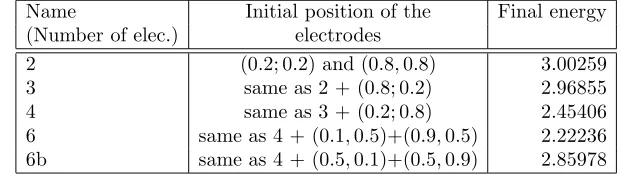
For the first serie of tests, the tumor is an ellipse with center [0.5,0.5] and semi-axis of sizes 0.2 and 0.3, in the directions xand y, respectively. The electrodes are disks of radius 0.02. The ponderation of the zone of interestχis equal to 10 in the tumor and 1 in the healthy tissue, meaning that we are 10 times more interested in satisfying the conditions inside the tumor than inside the healthy tissue. Several tests are performed with an increasing number of electrodes. Results are given in Table 1 and the optimal potential and electrodes placement is shown in Figure 1, whereas the convergence history is shown in Figure 2.

Name Initial position of the Final energy (Number of elec.) electrodes

2 (0.2; 0.2) and (0.8,0.8) 3.00259

3 same as 2 + (0.8; 0.2) 2.96855

4 same as 3 + (0.2; 0.8) 2.45406

6 same as 4 + (0.1,0.5)+(0.9,0.5) 2.22236 6b same as 4 + (0.5,0.1)+(0.5,0.9) 2.85978

Table 1. The initial position of the electrodes and the final value of the objective functionJ

for 2dtests.

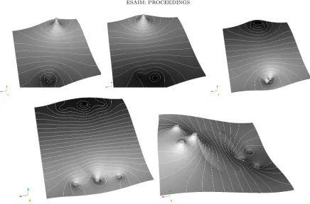
This 2d algorithm shows the right behavior. Generally, the more electrodes we use, the more degrees of freedom has the algorithm to optimize their positions. Tests 2 and 3 yield the same result, the added third electrode being useless and it is always “switch-off” during the optimization process, which means that it is always set to a potential that is the potential at the location of the electrode when it is removed.

Test 4 exhibits a two-step behavior. During iterations 1 to 5, it only optimizes the position of the two electrodes that are in location (0.2,0.2) and (0.8,0.8), switching off the other two electrodes. This can be seen in Figure 1 where the curve for 4 electrodes is similar to the one for 2 electrodes during the beginning of the optimization process. After having optimized the position of these two electrodes, it is concerned by two remaining ones, moving them slowly close to the tumor during iterations 10 to 22.

Figure 1. The electric potential for the optimal electrodes position in the 2d test. From left to right and from top to bottom, the number of electrodes is respectively 2,3,4,6,6b of Table 1

Figure 2. Convergence history of the objective function for the different electrodes in 2d case. Abscissa refers to the number of iterations.

The 3d tests are made on the cube Ω = [0,1]3_{meshed with aproximatively 35K tetrahedra. As for 2d tests,}

the electric potentials and the adjoint problem are solved using P1 finite elements and the conductivity σ,

represented with P0 finite elements, is equal to 0.4 in the healthy tissue and 1 in the tumor.

We consider a spherical tumor centered in (0.5,0.5,0.5) and with the diameter equals to 0.4. The electrodes are circular cylinders of diameter 0.1. The set of all possible electrodes configurations is subject to some restrictions : first of all electrodes have vertical position and the intersection with the plane of equationz= 1 is non-empty. Therefore, the three coordinates of the center of the lower base of the electrode describe completely its position.

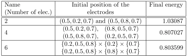
The ponderation of the zone of interest χ is equal to 10 in the tumor and 1 in the healthy tissue, meaning that we are 10 times more interested in satisfying the conditions inside the tumor than inside the healthy tissue. Several tests are performed with 2, 4 or 6 electrodes. Results are given in Table 2 and the optimal potential and electrodes placement is shown in Figure 3, whereas the convergence history is shown in Figure 4.

Name Initial position of the Final energy (Number of elec.) electrodes

2 (0.5,0.2,0.7) and (0.5,0.8,0.7) 1.03087

4 (0.5,0.2,0.7), (0.8,0.5,0.7)

(0.5,0.8,0.7), (0.2,0.5,0.7) 0.807027

6 {0.2,0.5,0.8} × {0.2} × {0.7}

{0.2,0.5,0.8} × {0.8} × {0.7} 0.803599

Table 2. The initial position of the electrodes and the final value of the objective function (sometimes called energy) in the 3dtests. The first column displays the number of electrodes.

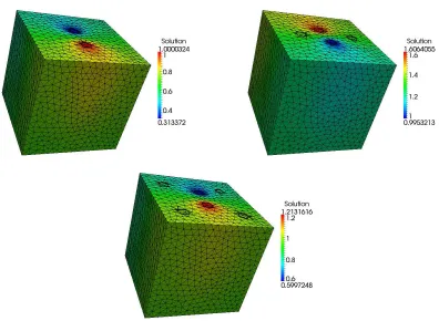
The results obtained in the 3d tests are similar to the results obtained in 2d. All the optimal configurations displayed in Figure 3 shows that, even for more than two electrodes, the energy is minimized by a pair of electrodes placed symmetrically around the tumor. This can be explained by the important size of the electrodes compared with the tumor.

6.

_Conclusion

Figure 3. The electric potential for the optimal placement of electrodes in 3d, with tests (from left to tight and top to bottom) number 2,4 and 6 of Table 2

0 5 10 15 20 25

0.8 1 1.2 1.4 1.6 1.8 2 2.2 2.4 2.6 2.8

Number of iterations

Energy

2 4 6

Figure 4. Convergence history of the objective function for the different numbers of electrodes in 3d case. Abscissa refers to the iteration number.

Acknowledgement

References

[1] Gr´egoire Allaire.Conception optimale de structures, volume 58 ofMath´ematiques & Applications (Berlin) [Mathematics & Applications]. Springer-Verlag, Berlin, 2007. With the collaboration of Marc Schoenauer (INRIA) in the writing of Chapter 8. [2] Jean C´ea. Conception optimale ou identification de formes: calcul rapide de la d´eriv´ee directionnelle de la fonction coˆut.

RAIRO Mod´el. Math. Anal. Num´er., 20(3):371–402, 1986.

[3] B. Gabriel and J. Teissi´e. Time courses of mammalian cell electropermeabilization observed by millisecond imaging of membrane property changes during the pulse.Biophys. J., 76:2158–2165 (electronic), 1999.

[4] C. Geuzaine and J. F. Remacle. Gmsh mesh generator.http://geuz.org/gmsh.

[5] M. Marty, G. Sersa, and J.-R. Garbayet al. Electrochemotherapy – an easy, highly effective and safe treatment of cutaneous and subcutaneous metastases: Results of esope (european standard operating procedures of electrochemotherapy) study.E.J.C Supplements, 4:3–13, 2006.

[6] Bertrand Maury. Numerical analysis of a finite element/volume penalty method. SIAM J. Numer. Anal., 47(2):1126–1148, 2009.

[7] F. Murat and S. Simon. ´etudes de probl`emes d’optimal design.Lecture Notes in Computer Science 41, Springer Verlag, pages 54–62, 1976.

[8] Y. Renard and J. Pommier. Getfem finite element library.http://home.gna.org/getfem.

[9] G. Serˇsa, D. Miklavˇciˇc, M. Cemazar, Z. Rudolf, G. Pucihar, and M. Snoj. Electrochemotherapy in treatment of tumours. EJSO. The Journal of Cancer Surgery, 34:232–240, 2008.

[10] S.I. Sukharev, V.A Klenchin, S.M. Serov, Chernomordik L.V., and Chizmadzhev Y.A. Electroporation and electrophoretic DNA transfer into cells: The effect of DNA interaction with electropores.Biophys J., 63:1320–1327, 1992.

[11] S. ˇCoroviˇc, J. Bester, and D. Miklavˇciˇc. An e-learning application on electrochemotherapy.BioMedical Engineering OnLine, 8, 2009.

[12] S. ˇCoroviˇc, M. Pavlin, and D. Miklavˇciˇc. Analytical and numerical quantification and comparison of the local electric field in the tissue for different electrode configurations.BioMedical Engineering OnLine, 6, 2007.

[13] M.C. Vernhes, P.A. Cabanes, and J. Teissi´e. Chinese hamster ovary cells sensitivity to localized electrical stresses. Bioelec-trochem. Bioenerg., 48:17–25, 1999.

[14] D. ˇSel, D. Cukjati, D. Batiuskaite, T. Slivnik, L.M. Mir, and D. Miklavˇciˇc. Sequential finite element model of tissue electrop-ermeabilization.IEEE Trans. Bio. Eng., 52(5):816–827, 2005.

[15] D. ˇSel, S. Mazeres, and D. Miklavˇciˇc. Finite-element modeling of needle electrodes in tissue from the perspective of frequent model computation.IEEE Trans. on BioMed. Eng., 50(11):1221–1232, 2003.