Definition of Probability Characteristics of the Absolute Maximum of Non-Gaussian Random Processes by Example of Hoyt Process

Published online May 30, 2013 (http://www.sciencepublishinggroup.com/j/ajtas) doi: 10.11648/j.ajtas.20130203.13

Definition of probability characteristics of the absolute

maximum of non-Gaussian random processes by

example of Hoyt process

O. V. Chernoyarov, A. V. Salnikova, Ya. A. Kupriyanova

Dept. of Radio engineering Devices of the National Research University “MPEI”, Moscow, Russia

Email address:

[email protected] (O. V. Chernoyarov)

To cite this article:

O. V. Chernoyarov, A. V. Salnikova, Ya. A. Kupriyanova. Definition of Probability Characteristics of the Absolute Maximum of Non-Gaussian Random Processes by Example of Hoyt Process. American Journal of Theoretical and Applied Statistics. Vol. 2, No. 3, 2013, pp. 54-60. doi: 10.11648/j.ajtas.20130203.13

Abstract:

The technique of a finding of distribution functions of an absolute maximum of non-Gaussian random processes has been illustrated. On an example of Hoyt process the limiting distribution laws of its absolute maximum have been found. By methods of statistical modeling it has been established that the given asymptotic approximations ensure a satisfactory description of the true distributions over a wide range of parameter values of the random process.

Keywords:

Differentiable and Nondifferentiable Random Process, Distribution Function of the Absolute Maximum, Outliers of the Random Process, Statistical Modeling

1. Introduction

The problem of distribution of the statistical characteristics of non-Gaussian random processes is widely used in various areas of a science and technics [1-5]. When analyzing the limiting deviations and stability of complex engineering systems and dealing with the reliability theory, construction mechanics, and the detection and communication theory we should know the distribution of the absolute (largest) maximum of the realization of the stationary random function [1-5]. Such problems as the description of the surface roughness during the mechanical conversion of parts, description of the rough sea surface, seismic and wind actions, analysis of vibrations, etc. are often reduced to the study of characteristics of maximum values. Among the most widely used non-Gaussian random functions the Hoyt process [6] can be singled out. This process is often named by under-Rayleigh process also [7] so far as signal fading at such model are deeper than Rayleigh fading. It is possible to formulate the Hoyt process as [6, 7]:

( )

t = N₁2

( )

t +N2₂

( )

t

η , t∈

[ ]

0;T . ₍₁₎

Here N_k

( )

t , k=1,2 are independent centered Gaussian random processes with variances σ2_k ≠0 and correlation

factors R

( )

τ so σ₁≠σ₂ in general. The one-dimensional probability density w_η

( )

x of the process η

( )

t have the form [6, 7]

( )

   

   

       

σ − σ

   

   

       

σ + σ − σ σ =

η ₂

2 2 1 2 0 2 2 2 1 2 2 1

1 1 4 x I 1 1 4 x exp x x

w , x≥0 (2)

where I0

( )

x _{is the modified Bessel function of zero order.} The examples of the process (1) are the module (amplitude) of scalar component of complex Gaussian field [6], the radio-signal fading under multipath propagation [7], the output signal of the optimal detector/measurer with dissymmetric quadrature channels [4, 5], the solving statistics in tasks of signal detection and measurement [8] and etc.

2. Distribution of the Absolute

Maximum of the Differentiable Hoyt

Process

Let us consider the normalized Hoyt process ~η

( )

t so following conditions are satisfied

( ) ( )

=η σ′ ηt t

~ _{, (3)}

( )

_

  

 

 _{χ +}

−     

 

 _{χ −}

χ =

η

4 1 x exp 4

1 x xI x w

2 2 2

2 0

~ , χ=σ′σ′′ (4)

which along with its first derivative

( )

t ~ ηɺ

is rms-continuous.

In Eqs. (3), (4) it is designated: σ′=max

(

σ1,σ2

)

_,

(

1, 2

)

minσ σ =

σ ′′ _{. In this case according to [2] for the}

correlation factor R

( )

τ of the quadratures N1,2

( )

t _the following relation is fulfilled when τ→0:

( )

2 2

( )

2

2 1

R τ = −α τ +οτ (5)

where

( )

2

τ

ο _{denotes the higher-order infinitesimal terms}

compared with τ2. Moreover, it is assumed that for τ→∞

( )

τ =ο

(

−1ατ

)

ln

R (6)

The quantity α in Eqs. (5) and (6) has a simple physical meaning. In the time domain it characterizes the correlation time τ_c of the processes N_1,2

( )

t . Indeed, confining ourselves to the parabolic approximation (5) of the function

( )

τ

R the correlation time can be determined τ_c as the duration of the function R

( )

τ at the level 0.5 [4, 5]. Then we have

α =

τ_c 2 . ₍₇₎

In the spectral domain the quantity α describes the equivalent width of the spectral density of the processes

( )

t N_1,2 [4, 5]:

( )

( )

12

2

d G d

G _

 

ω ω ω

ω ω =

α

_∫

_∫

∞

∞ − ∞

∞

− (8)

where

( )

∫

∞

( ) (

)

∞

− τ − ωτ τ

σ =

ω R exp j d

G 2 is the spectral

density of the processes N_1,2

( )

t . As it is obvious from [1, 2], once Eqs. (5) and (6) are fulfilled, the distribution of the number of outliers beyond the levelh of the process (1) is reduced to the Poisson law with increase ofh. Then for the desired probability

( )

h P

[

h h

]

F = _m< , h_m=sup

{

~η

( )

t :t∈

[ ]

0;T

}

(9)

we can write

[

h h

]

exp

[

( )

h

]

P lim _m

h < = −Π

→∞ ξ→∞

. ₍₁₀₎

Here

( )

( )

_

  

 

 _{χ +}

−

    

   _{χ −}

π ξχ = π ξ =

Π η

4 1 h exp 4

1 h I 2

h h w 2 h

2 2 2

2 0

~ (11)

is the average number of outliers of the process realization

( )

t

~

η beyond theh level over the interval

[ ]

0;T , w~_η

( )

h , χ are defined from Eq. (4), and

( )

= α ′′ − =

ξ T R 0 T (12)

is the referred length of the observation interval which characterizes the number of independent samples of the quadratures N_1,2

( )

t and the process ~η

( )

t [1].

In the general case the function on the right-hand side of Eq. (10) is not a nondecreasing function of h. Therefore, for an arbitrary h as an approximation for the distribution function of the absolute maximum of the process ~η

( )

t the following expression may be used

( )

[

( )

]

  

< ≥ Π

− ≈

, h h ,

0

, h h , h exp h

F

min min

(13)

where h_min is the minimum value of h, for which the inequality Π

( ) (

h >Π h+ε

)

is fulfilled for any ε>0. Due to the complex nature of the function (11) it is difficult to write the expression for h_min explicitly for σ₁≠σ₂ . However, calculating the values of h_min for different χ by using numerical methods it is possible to see that approximation

( )

χ =2

(

1+χ

)

h_min (14)

can be used without conspicuous loss of accuracy.

Expression (13) of the distribution of maximum values is approximate but its accuracy increases withh and ξ [1, 2, 5]. For smallh and ξ the approximation (13) may be very rough. Since for T→0 (ξ→0) the distribution of the maximum value of the process ~η

( )

t (3) is limited to the Hoyt distribution it can be used the approximation of the

type [4, 5] where _η

( )

=

∫

h _η

( )

0 ~

~ h w x dx

F is Hoyt distribution

function. Unlike Eq. (13), the approximation (15) is asymptotically accurate not only for ξ→∞ but also for

0 →

random process with a one-sided Gaussian distribution.

( )

( )

( )

     

      

 

< 

       

 

 _{χ +}

− ×

× 

  

    

 

 _{χ −}

π ξχ −

≥ 

       

 

 _{χ +}

− ×

× 

  

    

 

 _{χ −}

π ξχ

≈

η η

, h h ,

4 1 h

exp

4 1 h

I 2 h exp h F

, h h ,

4 1 h exp

4 1 h I 2

h exp h F

h F

min 2

2 min

2 2 min 0 min ~

min 2

2

2 2 0 ~

1

₍₁₅₎

The possibility of using Eq. (15) for calculating the characteristics of the absolute maxima of finite-duration realizations of the Hoyt random process was investigated with the help of statistical computer modeling. It was assumed that R

( )

τ =exp

(

−α2τ2 2

)

. In the process of modeling with step ∆ over the interval

[ ]

0;1 the samples of realizations of the normalized random process ~η

( )

~t (3) were generated in the normalized time scale ~t =t T:

( )

j 12

( )

j 2 22

( )

tj ~ N~ t ~ N~ t ~

~ _{= +χ}

η , k

( ) ( )

k t k

~ N t ~

N~ = σ , k=1,2. (16)

The samples of processes N~_1,2

( )

~t were formed on the basis of a sequence of independent Gaussian numbers using the moving summation method [9]

( )

∑

−

= −

= p

p i

i j , k i j

k t cx

~

N~ , k=1,2. (17)

Here c_i =

(

2ξ2∆2 π

)

14exp

(

−i2ξ2∆2

)

, and x_k,i are independent Gaussian random numbers with zero math-ematical expectation and unit variance.

Parameters ∆ and p were chosen such that the rms error of the stepwise approximation (17) of a continuous realization of the processes N~_k

( )

~t , k=1,2 would not exceed 5%. In the experiment described it was ∆=0,01ξ,

200

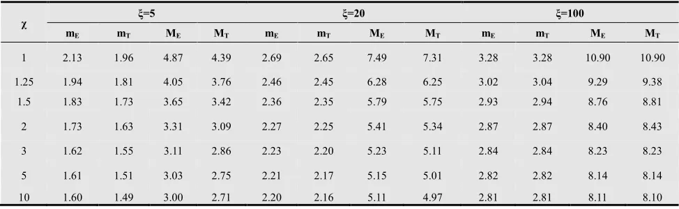
p= . In each realization a maximum h_m had been founded. Using all the N realizations (N=2⋅105) the empirical average value m_E, the mean square M_E, and the values of the distribution functions of the absolute maxima for differenthand ξ had been calculated.

In Table 1 the modeled mE and ME as well as the corresponding theoretical characteristics

( )

[

]

∫

∞ η

− =

0 ~

T 1 F h dh

m ,

∫

[

( )

]

∞ η

− =

0 ~ T 2 h1 F h dh

M (18)

calculated by numerical methods using Eq. (15) are shown. From Table 1 it is obvious that the accuracy of the approximate formula (15) is improved with increasing ξ.

Table 1. Theoretical and experimental values of first two moments of distribution of an absolute maximum of differentiable Hoyt process

χ ξ=5 ξ=20 ξ=100

mE mT ME MT mE mT ME MT mE mT ME MT

1 2.13 1.96 4.87 4.39 2.69 2.65 7.49 7.31 3.28 3.28 10.90 10.90

1.25 1.94 1.81 4.05 3.76 2.46 2.45 6.28 6.25 3.02 3.04 9.29 9.38

1.5 1.83 1.73 3.65 3.42 2.36 2.35 5.79 5.75 2.93 2.94 8.76 8.81

2 1.73 1.63 3.31 3.09 2.27 2.25 5.41 5.34 2.87 2.87 8.40 8.43

3 1.62 1.55 3.11 2.86 2.23 2.20 5.23 5.11 2.84 2.84 8.23 8.23

5 1.61 1.51 3.03 2.75 2.21 2.17 5.15 5.01 2.82 2.82 8.14 8.14

10 1.60 1.49 3.00 2.71 2.20 2.16 5.11 4.97 2.81 2.81 8.11 8.10

In Figs. 1 the theoretical and experimental distribution functions of the absolute maximum of the differentiable Hoyt random process are drown. The solid curves in Fig. 1a denote theoretical dependences F₁

( )

h obtained for χ=1 using Eq. (15), while the dashed curves indicate the same for χ=2. The solid curves in Fig. 1b show similar dependences for χ=3, while the dashed curves show the same for χ=10. Curves 1 correspond to ξ=5, curves 2 to ξ=20, and curves 3 to ξ=100. In Figs. 1 and 2 the experimental values of the distribution function for ξ=5, 20 and 100 are denoted by rectangles, crosses, and

diamonds (for χ=1 and χ=3), respectively, as well as by plus signs, circles and triangles (for χ=2 and

10 =

χ ).

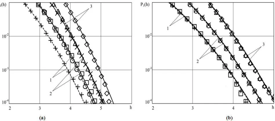
Since in a number of tasks it is necessary to know the behavior of the tails of the distribution function, in Figs. 2 the probabilities P₁

( )

h =1−F₁

( )

h for largeh under ξ=5, 20, 100 and χ=1, 2 (Fig. 2a) or χ=3, 10 (Fig. 2b) are shown. The notations in Figs. 2 correspond to those used in Figs. 1.

differentiable Hoyt process η

( )

t (1) approximates the experimental results in a satisfactory manner, at least, for

5 ≥

ξ and h≥h_min.

Figure 1. The theoretical and experimental dependences of distribution functions of the absolute maximum of the differentiable Hoyt random process.

Figure 2. The theoretical and experimental dependences of the tails of the distribution functions of the absolute maximum of the differentiable Hoyt random

process

3. Distribution of the Absolute

Maximum of the Nondifferentiable

Hoyt process

Let us consider the nondifferentiable Hoyt process ~η

( )

t (3). By analogy with [4] it is assumed that the following relation is fulfilled for the correlation factor R

( )

τ of the quadratures N_1,2

( )

t under τ→0:

( )

τ =1−δ τ+ο

( )

τ

R , δ>0 (19)

while under τ→∞ we have R

( )

τ =ο

(

ln−1δτ

)

. The quantity δ, as the α in Eq. (5), determines the

correlation-spectral properties of the processes N_1,2

( )

t . By analogy with Eq. (7), assuming that the correlation time τ_c is equal to the duration of the triangular approximation (19) of the function τ_c at the level 0.5, we obtain τ_c =δ−1. Because of the nondifferentiability of the quadratures

( )

t

N_1,2 it is impossible to determine the equivalent width of the spectral density in accordance with Eq. (8). However, to describe the length of the spectral density G

( )

ω along the frequency axis, we can use one of the definitions of the effective width of the spectral density ∆fe [1], for example,

( )

∫

( )

∞

∞

− π

ω ω ω

= ∆

2 d G G

max 1

It should be noted that the effective width of the spectral density is directly proportional toδ. _{Thus for the exponential}

correlation factor

( )

τ =exp

( )

−δτ

R (21)

of the random processes N_1,2

( )

t from Eq. (20) we have 2

f_e =δ

∆ .

From Eq. (19) it is obvious that the quadratures N_1,2

( )

t are the Gaussian locally-Markov random processes [10]. However, for arbitrary time intervals the Markov properties of the processes N_1,2

( )

t are preserved only when the correlation factor R

( )

τ satisfies the relation (20) [3].

In accordance with [1, 4] fulfilling (21) and the conditions

2 1<<σ

σ , σ₁>>σ₂ or σ₁ ≈σ₂ , we approximately assume the process η

( )

t to be the Markov random process. In the general case for arbitrary σ₁, σ₂ the Markov behavior of the process η

( )

t can be violated. However, using the local Markov properties of the quadratures N_1,2

( )

t it is possible to show that on fulfillment of Eq. (19) the process η

( )

t (1) can be approximately considered by locally-Markov Hoyt process with the stationary distribution law (2). In this case the realizations of the processes N_1,2

( )

t and η

( )

t are continuous with probability 1 as in the realizations of the diffusion-type Markov processes.

In accordance with [4] the probability characteristics of an excess over a sufficiently high level match asymptotically for the Markov and locally-Markov processes. Indeed, due to the continuous behavior of realizations of the Markov and locally-Markov processes the duration of the segments at which the realizations exceed a certain levelhtends to zero as h→∞ . Therefore, for h→∞ the level h is not exceeded with probability determined only by the local properties of the process. Then, using the results of [3, 4] we write the following expression for the probability as in Eq. (9):

[

h h

]

exp

(

T

)

P _m < ≈ −ρ , (22)

where

( )

∫

δ = ρ h

x0wst x dx 1 1

(23)

and w_st

( )

x is the stationary probability density of the normalized random process ~η

( )

t (3) which is determined from Eq. (4). Equation (22) was obtained in [3] for the case

1 m>> and

( )

h 1

w_st << . (24)

Here m=δT is the referred length of the observation interval, which characterizes the number of independent samples of the processes N_1,2

( )

t and η

( )

t similarly to ξ in

Eq. (12). Obviously, the condition (24) holds for the Hoyt process when h>>1. The value of x₀ in Eq. (23) is chosen in the region of maximum probability of the process values ~η

( )

t , so that we can assume that x₀ =2

(

1+χ

)

. Then, using the asymptotic Laplace formula [11] for evaluating the integral (23), we obtain the following expression for h→∞:

( )

[

]

( )

[

2 2

]

[

( )

1

]

0 2 2 h 1 4 1 h DI 4 1 h exp 1 1 ₋ Ο + − χ + χ δχ = ρ (25)

( )

(

)

( )

(

)

1

4 1 h I 4 1 h I 2 1 2 1 h D 2 2 0 2 2 1 2 2 2 ₋         − χ − χ − χ − + χ =

where Ο

( )

h−1 denotes terms of order 1h, and I₁

( )

x is the modified Bessel function of first order. Therefore, for large h in accordance with Eqs. (22) and (25) we write the following expression for the probability as in Eq. (9):

[

h h

]

exp

[

m

( )

h

]

P _m< ≈ − ϕ (26)

where

( )

(

)

(

)

( )

(

)

( )

(

)

1 .

4 1 h I 4 1 h I 2 1 2 1 h 4 1 h exp 4 1 h I h 2 2 0 2 2 1 2 2 2 2 2 2 2 0         −         − χ − χ − χ − + χ × ×       

 _{χ +}

−       

 _{χ −}

= ϕ

In this case as is obvious from [3] the accuracy of the approximate formula (26) increases withm andh.

Since the right-hand side of Eq. (26) is a nondecreasing function only for h≥h_min for the distribution function of the absolute maximum of the process ~η

( )

t we use the approximation

( )

[

( )

]

   < ≥ ϕ − = , h h , 0 , h h , h m exp h F min min (27)

where h_min is the minimum value of h for which the inequality ϕ

( ) (

h >ϕh+ε

)

holds for any ε>0. For a fixed

1 ≠

χ the quantity hmin can be calculated using only numerical methods. However, by analogy with Eq. (14) for the function h_min =h_min

( )

χ without significant loss of accuracy we propose the approximation

17 . 2

min 3 2

h = +χ . (28)

( )

( )

[

( )

]

[

( )

]

( )

(

)

( )

(

)

( )

[

( )

]

[

( )

]

( )

(

)

( )

(

)

     

      

 

<     

  

−     

  

− χ

− χ −

χ − + χ ×

× + χ − −

χ

≥     

  

−     

  

− χ

− χ −

χ − + χ ×

× + χ − −

χ

=

η η

. h h

, 1 4 1 h

I

4 1 h

I 2

1 2

1 h

4 1 h

exp 4 1 h

I h F

, h h

, 1 4 1 h I

4 1 h I 2

1 2

1 h

4 1 h exp 4 1 h I h F

h F

min 2

2 min 0

2 2 min 1 2 2 2 min

2 2 min 2

2 min 0 ~

min 2

2 0

2 2 1 2 2 2

2 2 2

2 0 ~

1

(29)

Unlike Eq. (27), the approximation (29) is asymptotically accurate for both m→∞ and m→0. For largeh and m the approximations (27) and (29) in practice coincide. Besides, for χ=1 the distribution function F₁

( )

h (29) corresponds to the distribution function of the absolute maximum of the Rayleigh random process and for χ>>1 – to the distribution function of the absolute maximum of the random process with a one-sided Gaussian distribution.

The possibility of using Eq. (29) it was investigated with the help of computer modeling of the normalized Hoyt

process (3) with the correlation factor of the quadratures (21). The modeling of the nondifferentiable process ~η

( )

t (3) was performed by analogy with the above described modeling of the differentiable process. The difference is that in forming the samples of the normalized Gaussian processes N~_1,2

( )

~t the recurrent method in order to reduce computer time had been used [9]:

( )

( )

k,j

( )

k

( )

j1 2

j

k t

~ N~ R~ x R~ 1 t ~

N~ = − ∆ + ∆ ₋ , k=1,2.

Here R~

( )

∆ =exp

(

−m∆

)

, and xk,j are independent Gaussian numbers with zero mathematical expectation and unit variance. The discretization step ∆=0,02 m was chosen to ensure an rms error below 5% when reproducing the realization N~_1,2

( )

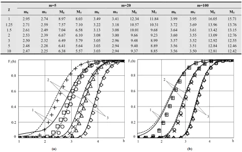
~t .

In Table 2 the m_E and M_E resulting from the modeling as well as the m_T and M_T calculated from Eqs. (18) and (29) are shown. From Table 2 it is obvious that the accuracy of the approximate formula (29) increases with increasing m.

Table 2. Theoretical and experimental values of first two moments of distribution of an absolute maximum of nondifferentiable Hoyt process

χ m=5 m=20 m=100

mE mT ME MT mE mT ME MT mE mT ME MT

1 2.95 2.74 8.97 8.03 3.49 3.41 12.34 11.84 3.99 3.95 16.05 15.71

1.25 2.71 2.59 7.57 7.10 3.22 3.18 10.57 10.31 3.72 3.69 13.96 13.76

1.5 2.61 2.49 7.04 6.58 3.13 3.08 10.01 9.68 3.64 3.61 13.42 13.15

2 2.53 2.39 6.67 6.10 3.08 3.00 9.66 9.23 3.60 3.55 13.09 12.76

3 2.50 2.32 6.49 5.79 3.05 2.96 9.48 8.99 3.57 3.52 12.92 12.55

5 2.48 2.28 6.41 5.64 3.03 2.94 9.40 8.89 3.56 3.51 12.84 12.46

10 2.47 2.25 6.38 5.57 3.03 2.94 9.37 8.85 3.56 3.50 12.81 12.42

Figure 3. The theoretical and experimental dependences of distribution functions of the absolute maximum of the nondifferentiable Hoyt random process.

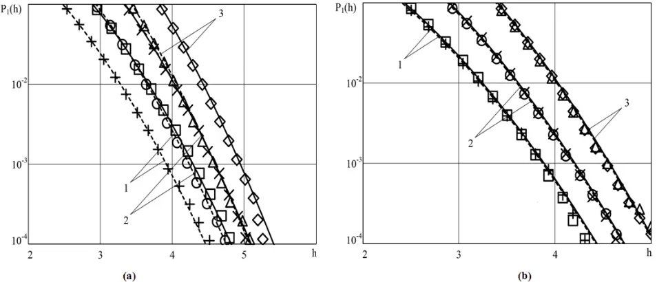
In Figs. 3 the theoretical and experimental dependences

( )

h

F₁ are shown, while in Fig. 4 the dependences

( )

h 1 F

( )

h

P₁ = − ₁ for the nondifferentiable Hoyt process are presented. The solid curves denote theoretical dependences calculated from Eq. (29) for χ=1 (Figs. 3a and 4a) or

3 =

χ (Figs. 3b and 4b), while the dashed curves represent the same dependences for χ=2 (Figs. 3a and 4a) or

10 =

χ (Figs. 3b and 4b).

Curves 1 correspond to m=5, curves 2 correspond to

20

Experimental values of the probability F₁

( )

h or P₁

( )

h for 5

m= , 20, and 100 are shown in Figs. 3, 4 by rectangles, crosses, and diamonds (for χ=0.5 and χ=5 ), respectively, as well as by plus signs, circles and triangles (for χ=2 and χ=10 ). All the experimental characteristics of the nondifferentiable process were obtained as a result of the processing of N=2⋅105

realizations of the random process ~η

( )

~t .

From Figs. 3, 4 it is obvious that the asymptotically exact expressions (29) for the distribution function of the absolute maximum of the nondifferentiable Hoyt process η

( )

t (1) satisfactorily approximate the experimental data, at least, for

5

m≥ and h≥h_min.

Figure 4. The theoretical and experimental dependences of the tails of the distribution functions of the absolute maximum of the nondifferentiable Hoyt

random process

4. Conclusion

To calculate the characteristics of the maximum values of random processes the limiting distribution laws of the absolute maximum obtained for the case of an unlimited increase of the values of maxima and the duration of realizations can be used. The form of asymptotic approximations depends on the analytical properties of the process, namely, on the existence of its continuous derivative. Performing the comparison with the experimental data exemplificative of Hoyt process it is possible to see that the offered technique allows to receive the asymptotic formulas which ensure a satisfactory description of the true distributions over a wide range of parameter values of the random process.

Acknowledgements

The reported study was supported by Russian Foundation for Basic Research, research project No. 13-08-00735a.

References

[1] V.I. Tikhonov, V.I. Khimenko, Outliers of Random Process Trajectories [in Russian]. Moscow: Nauka, 1987.

[2] H. Cramer, V. Leadbetter, Stationary and Related Stochastic

Processes. New York: Wiley, 1967.

[3] R.L. Stratonovich,Selected Problems of Fluctuation Theory in Radio Engineering [in Russian]. Moscow: Sovetskoe Radio, 1961.

[4] Signal detection theory[in Russian]. Moscow: Radio i Svyaz', 1984.

[5] A.P. Trifonov, Yu.S. Shinakov, Joint Discrimination of Signals and Estimation of their Parameters against Background [in Russian]. Moscow: Radio i Svyaz', 1986. [6] R.S. Hoyt, “Probability functions for modulus and angle of

the normal complex variate”, BSTJ, 1947, vol. 26, no. 2, p. 318-359.

[7] D.D. Klovsky, Discrete message passing on radio channels [in Russian]. Moscow: Radio i Svyaz', 1982.

[8] O.V. Chernoyarov The statistical analysis of random pulse signals against hindrances under conditions of various prior uncertainty [in Russian] // D.Sc. Thesis. Moscow: Moscow Pedagogical State University, 2011.

[9] V.V. Bykov, Numerical Modeling in Statistical Radio Engineering [in Russian]. Moscow: Sovetskoe Radio, 1971. [10] J.A. McFadden, “On a class of Gaussian process for which

the mean rate of crossing is infinite”, J. Roy. Statist. Soc. Ser. B., 1967, vol. 29, no. 3, p. 489-502.