Korets M.A.
a*, Prokushkin A.S.
aa Sukachev Institute of Forest Siberian Branch, Russian Academy of Science, [email protected], [email protected] * Corresponding author
Abstract: The depth of the active layer is highly valuable parameter of the biochemical processes and ecosystem dynamics in changing climate. Site area of our investigation was situated in the Evenkiysky District of Krasnoyarsk Krai, Russia near Tura settlement. We used field measurements of seasonal thawing layer depth (active layer depth) to estimate its spatial variability and its dependency of topography-based variables (elevation, slope and aspect). The spatial analysis of field sample plots location and after-forest-fire period length helped us to build the reference table and then extrapolate this data in a form of map for the site area. The produced map of active layer depth and applied data processing scheme are now using for the complex analysis and modelling of hydrochemical processes in terrain- and water-ecosystems.
Keywords: GIS, Thematic maps, Permafrost active layer depth, DEM
1. Introduction
The active layer is a surface part of the permafrost, that freezes and thaws each year. Therefore, the ddepth of the active layer is highly valuable parameter of the biochemical processes and ecosystem dynamics in changing climate.
We planned to use the active layer depth map for the analysis of biomass and carbon transformation processes in terrain- and water-ecosystems (Prokuskin et al., 2006, 2011) as a part of ongoing projects (see Acknowledgements). One of the corresponding subtask was to estimate the dependence of carbon stock value of the organic layer per test watersheds and seasonal thawing layer depth.
We used the local GIS-based data bank, including topographic site layers, digital elevation model (DEM), field sites forest inventory database, remote sensing (RS) satellite data, and input/resulting thematic maps of vegetation parameters (Korets et al., 2016).
Classification and inventory of the current diversity of forest communities and their environments (i.e. site conditions) were developed for Northern Siberia test site (area ~360 000 ha), situated in the Evenkiysky District of Krasnoyarsk Krai, Russia near Tura settlement (N64°17’, E100°13’). This classification considers characteristics of forest regeneration dynamics, such as trends and rates of forest regeneration succession in a range of site conditions; therefore, we used this conception as a basis for terrestrial ecosystem mapping. An algorithm of forest regeneration dynamics mapping based on a spatial analysis of multi-band satellite data, a digital elevation model, and ground truth data combined with expert estimates of the resulting land cover classes was applied
(Korets et al., 2016). According this approach we used the automated classification of RS-based (spectral reflectance) and DEM-based (elevation, slope and modified exposition) to map forest regeneration series and site conditions for the Tura test site area. Based on this algorithm, Landsat TM/ETM/OLI satellite imagery, ASTER GDEM, and field data were processed for the test site area.
The field measurements data (Prokuskin et al., 2006) and above maps, available for the Tura site, incorporated in the GIS database allowed us to extrapolate and map the biomass and carbon pools values (kgC/m2), using
combined (spatially intersected) layers of vegetation growing condition and landcover.
The above thematic layers, including DEM (elevation above sea level, aspect angle, and slope angle), RS-based maps (burned areas after forest fire), carbon pools values, and streams watersheds polygons provided the basis for the further data processing.
2. Data processing and mapping
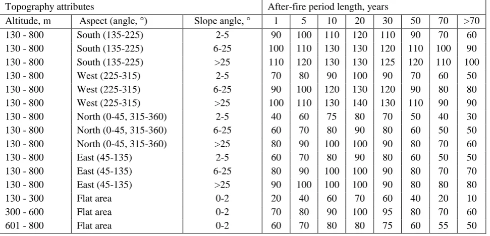
We used field sample measurements (2006 - 2015) of seasonal thawing layer depth (active layer depth) to estimate its spatial variability and dependency to local condition parameters. The spatial analysis of local site condition attributes (elevation, slope and aspect) and after-fire period length helped us to build the reference table (Table 1, Prokushkin et al., 2011) and extrapolate its data for the Tura local site area (Figure 1).
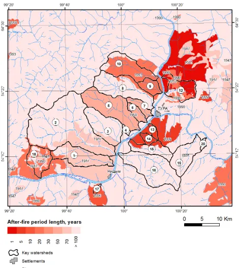
The map of burned forest areas was built by satellite imagery (Landsat MSS/TM/OLI, 1980 - 2013) processing together with Global Forest Change Map (Hansen et al.,
2013) and retrospective state forest inventory data of 1960.
Topography attributes After-fire period length, years
Altitude, m Aspect (angle, °) Slope angle, ° 1 5 10 20 30 50 70 >70 130 - 800 South (135-225) 2-5 90 100 110 120 110 90 70 60 130 - 800 South (135-225) 6-25 100 110 130 130 120 110 100 90 130 - 800 South (135-225) >25 110 120 130 130 125 120 110 100 130 - 800 West (225-315) 2-5 70 80 90 100 90 70 60 50 130 - 800 West (225-315) 6-25 90 100 120 130 120 90 80 80 130 - 800 West (225-315) >25 100 110 130 140 130 110 90 90 130 - 800 North (0-45, 315-360) 2-5 40 60 75 80 70 50 40 30 130 - 800 North (0-45, 315-360) 6-25 60 70 80 90 80 60 50 50 130 - 800 North (0-45, 315-360) >25 80 90 100 100 90 80 70 60 130 - 800 East (45-135) 2-5 60 70 80 90 80 60 50 50 130 - 800 East (45-135) 6-25 80 90 100 100 90 80 70 70 130 - 800 East (45-135) >25 90 100 100 100 90 80 80 80
130 - 300 Flat area 0-2 20 40 60 70 60 40 20 10
300 - 600 Flat area 0-2 70 80 90 100 95 80 70 60
601 - 800 Flat area 0-2 60 70 80 80 75 60 55 50
Table 1. The seasonal thawing layer depth (cm, bold numbers)
Then we classified DEM-based raster layers (altitude, aspect and slope angle) according the reference-table intervals (Table 1) and converted the resulting layers to vector polygons labeled by reference interval names. The layer of burned areas polygons was labeled by after-fire period length.
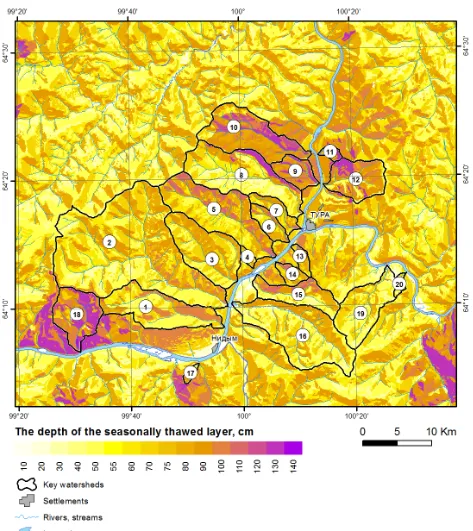
Finally, we overlaid and spatially intersected four polygonal layers to produce new polygons with all possible attributes combinations, provided by active layer depth values from reference-table. The resulting map of seasonal thawing layer depth for the Tura local site area is shown on Figure 3.
3. Conclusions
This paper demonstrate the application of typical GIS-based approach for spatial analysis, data interpolation and mapping. Using the GIS-based procedures of spatial intersection for the input layers: relief altitude, slope and aspect intervals, after-fire age intervals (for burned forest areas) and field reference data, we built the output map of seasonal thawing layer depth.
The produced map and applied data processing scheme
4. Acknowledgements
This study was started in the framework of the grant by Ministry of Education and Science of Russian Federation №14.B25.31.0031 and involved to the projects of Russian Foundation for Basic Research № 05-60203, № 18-05-00235, and 18-05-00781).
5. References
Hansen M. C., Potapov P. V., Moore R., et al. (2013). High-Resolution Global Maps of 21st-Century Forest Cover Change. Report. Science, 15 Nov 2013: Vol. 342, Issue 6160, pp. 850-853, DOI: 10.1126/science.1244693 Korets, M. A., Ryzhkova, V. A., Danilova, I. V., and Prokushkin, A. S. (2016). Vegetation cover mapping based on remote sensing and digital elevation model data. Int. Arch. Photogramm. Remote Sens. Spatial Inf. Sci., XLI-B8, 699-704, doi:10.5194/isprs-archives-XLI-B8-699-2016
Figure. 2. Burned areas of different ages (Tura local site), mapped by Landsat MSS/TM/OLI imagery (1980 – 2013), Global Forest Change Map (Hansen et al., 2013) and old forest inventory data (1960).
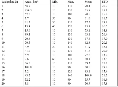
Figure. 4. Seasonal thawing layer depth vs carbon stock value of the organic layer per key watershed areas (points and labels).
Watershed № Area , km2 Min. Max. Mean STD
1 68.7 10 130 70.4 20.7
2 254.3 10 130 65.9 18.1
3 67.6 10 100 70.5 15.8
4 3.7 50 90 61.6 11.7
5 91.7 30 110 77.5 19.8
6 15.4 40 120 75.7 16.5
7 15.6 10 110 73.1 14.8
8 89.1 10 130 63.1 26.4
9 20.8 10 130 97.6 17.0
10 70.5 10 140 92.8 20.1
11 4.9 20 130 81.9 16.1
12 41.0 10 130 81.8 20.9
13 6.9 10 100 77.6 13.2
14 9.6 60 120 80.1 13.3
15 36.0 10 110 69.3 25.2
16 102.8 10 90 60.6 19.8
17 3.2 10 120 83.1 15.4
1 2 3 4 5 6 7 8 9 10 11 12 13 14 15 16 17 18 19 20
R² = 0.6264
40.0 50.0 60.0 70.0 80.0 90.0 100.0 110.0
0.60 0.70 0.80 0.90 1.00 1.10 1.20 1.30 1.40 1.50 1.60
Th e sea so n al th awin g la yer d ep th , cm
Carbon stock value of the orgnic layer, kgC/m2