Advanced regression and detection methods for remote sensing data analysis

(1)

International Doctorate School in Information and Communication Technologies

DISI - University of Trento

Advanced regression and detection methods for

remote sensing data analysis

Davide Castelletti

Advisor:

Lorenzo Bruzzone

Co-advisor:

Beg¨um Demir

(2)

(3)

Nowadays the analysis of remote sensing data for environmental monitoring is funda-mental to understand the local and global Earth dynamics. In this context, the main goal of this thesis is to present novel signal processing methods for the estimation of biophysical parameters and for the analysis icy terrain with active sensors. The thesis presents three main contributions.

In the context of biophysical parameters estimation we focus on regression methods. According to the analysis of the literature, most of the regression techniques require a rel-evant number of reference samples to model a robust regression function. However, in real-word applications the ground truth observations are limited as their collection leads to high operational cost. Moreover, the availability of biased samples may result in low estimation accuracy. To address these issues, in this thesis we propose two novel contribu-tions. The first contribution is a method for the estimation of biophysical parameters that integrates theoretical models with empirical observations associated to a small number of in-situ reference samples. The proposed method computes and correct deviations between estimates obtained through the inversion of theoretical models and empirical observations. The second contribution is a semisupervised learning (SSL) method for regression defined in the context of the ε-insensitive SVR. The proposed SSL method aims to mitigate the problems of small-sized biased training sets by injecting priors information in the initial learning of the SVR function, and jointly exploiting labeled and unlabeled samples in the learning phase of the SVR.

The third contribution of this dissertation addresses the clutter detection problem in radar sounder (RS) data. The capability to detect clutter is fundamental for the inter-pretation of subsurface features in the radargram. In the state of the art, techniques that require accurate information on the surface topography or approaches that exploit com-plex multi-channel radar sounder systems have been presented. In this thesis, we propose a novel method for clutter detection that is independent from ancillary information and limits the hardware complexity of the radar system. The method relies on the interferomet-ric analysis of two-channel RS data and discriminates the clutter and subsurface echoes by modeling the theoretical phase difference between the cross-track antennas of the RS. This allows the comparison of the phase difference distributions of real and simulated data.

(4)

Keywords[Remote sensing, signal processing, biophysical parameters estimation, sup-port vector regression, synthetic aperture radar, radar sounder, clutter detection.]

(5)

(6)

List of Tables

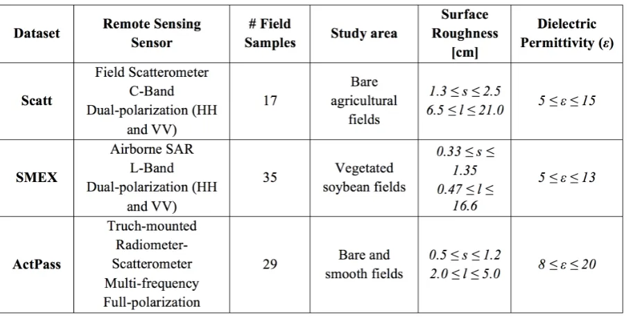
3.1 Main characteristics of the three datasets considered in the experimental analysis. . . 35

3.2 Estimation performances obtained by the proposed hybrid approach with the GDB and LDB strategies and the standard inverse theoretical model (Scatt dataset). . . 37

3.3 Estimation performances obtained by the proposed hybrid approach with the GDB and LDB strategies and the standard inverse theoretical model (SMEX dataset). . . 39

3.4 Estimation performances obtained by the proposed hybrid approach with the GDB and LDB strategies and the standard inverse theoretical model (ActPass dataset). . . 41

4.1 The list of variables used in the experiments and their physical meanings for the estimation of stem diameter. . . 58

4.2 The list of variables used in the experiments and their physical meanings for the estimation of abalones ages. . . 59

4.3 Mean and standard deviation (std) of MAE and R2 obtained by the stan-dard SVR and proposed SS-SVR. . . 61

4.4 Results of the first step of proposed method obtained when the value of radius is estimated either by the proposed strategy or by randomly fixing its value. . . 61

4.5 Mean and standard deviation (std) of MAE and R2 _{obtained by executing}

the proposed SS-SVR with and without the 2nd step. . . 62

4.6 Mean and standard deviation (std) of MAE and R2 _{obtained by the}

stan-dard SVR and proposed SS-SVR. . . 63

4.7 Comparison of the results of the first step of proposed method obtained when the value of radius is estimated by either the proposed strategy or by randomly fixing its value. . . 63

(11)

5.1 Typical operating parameters for MARFA RS. . . 79 5.2 SAD obtained between the real and the simulated (on both nadir and

clutter hypothesis) histograms and mean of the simulated distributions. . . 82 5.3 SAD obtained on real and simulated (on both nadir and clutter hypothesis)

histograms and mean of the simulated distributions for the selected feature. 85 5.4 SAD values obtained between the real and the simulated (on both nadir and

clutter hypothesis) histograms and the mean of the simulated distributions for feature f1. . . 89

5.5 SAD values obtained between the real and the simulated (on both nadir and clutter hypothesis) histograms and mean of the simulated distributions for feature f2. . . 89

(12)

List of Figures

2.1 Monostatic radar configuration. . . 10

2.2 Principle of SAR. . . 11

2.3 SAR acquisition geometry. . . 12

2.4 Interferometric radar configurations. . . 15

2.5 Exact formula of the interferometric phase in the cross-track single-pass configuration. . . 16

2.6 Nadir acquisition geometry of radar sounder systems. . . 17

2.7 Geometry of the clutter problem. . . 23

2.8 Surface clutter contribution before SAR processing (light gray locus), and after focusing in azimuth direction by Doppler processing and in range by range compression (dark gray cells). This example assumes flat topography in the absence of airplane roll. . . 24

3.1 Block diagram of the proposed hybrid approach. . . 31

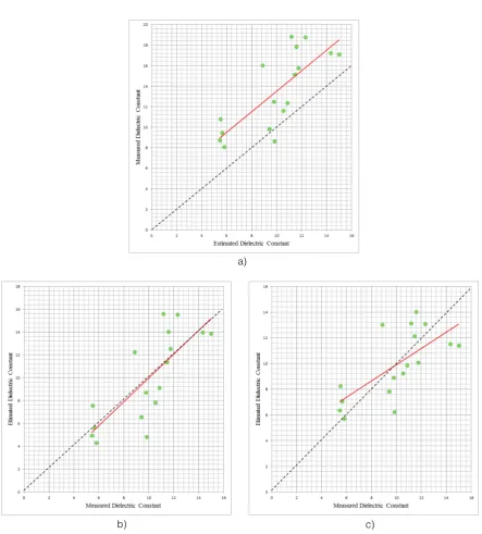
3.2 Scatterplots of measured versus estimated dielectric constant values ob-tained by (a) the inverse theoretical model, (b) the proposed hybrid ap-proach with the GDB strategy, and (c) the proposed hybrid apap-proach with the LDB strategy (Scatt dataset with HH23 features). . . 38

3.3 Scatterplots of measured versus estimated dielectric constant values ob-tained by (a) the inverse theoretical model, (b) the proposed hybrid ap-proach with the GDB strategy, and (c) the proposed hybrid apap-proach with the LDB strategy (SMEX dataset). . . 40

3.4 Scatterplots of measured versus estimated dielectric constant values ob-tained by (a) the inverse theoretical model, (b) the proposed hybrid ap-proach with the GDB strategy, and (c) the proposed hybrid apap-proach with the LDB strategy (ActPass dataset with the HHVV feature). . . 42

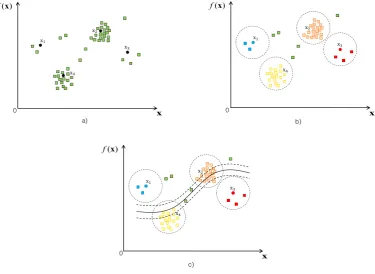
4.1 Block scheme of the proposed SSL method. . . 51

(13)

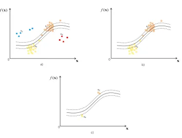
ples are the circles in black. b) Radius definition to estimate the weight of label samples. c) the WSVR learning function. . . 53 4.3 A qualitative example in a 1-D feature space. (a) the WSVR learning

function obtained at the first step; (b) selection of SVs that lie on the ε -tube after elimination of samples out and far from the -tube (c) selection of informative unlabeled samples having largest confidence and relevancy to be correctly estimated. . . 57

5.1 2-D representation of the acquisition geometry of a RS instrument. . . 70 5.2 Block diagram of the proposed technique. . . 71 5.3 Example of manual feature selection. a) The red area corresponds to the

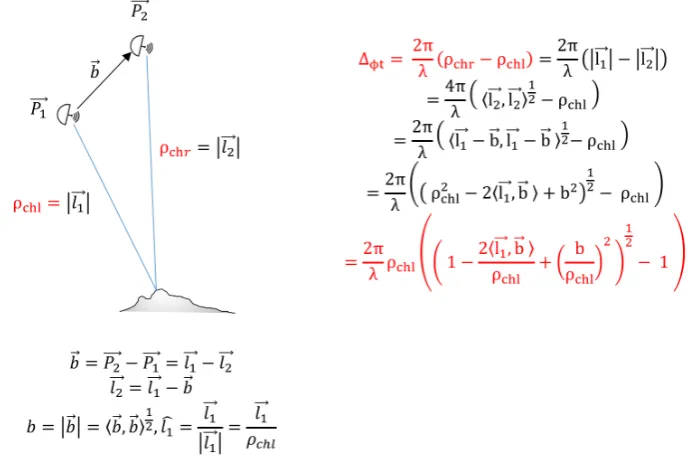
set of pixels that belong to a feature of interest. b) The yellow line is the simple feature-model used to project the feature onto the surface in the cross-track direction. . . 72 5.4 Two-channel sounding geometry. The red dots are reflection points on the

surface. For echoes coming from nadir, the signal path length ρchl andρchr are equivalent and ∆Φt = 0. The red dotted line represents an example of off-nadir signal path (for a clutter feature with the same delay), in which the difference between ρchl and ρchr makes ∆Φt 6= 0. . . 73 5.5 Qualitative illustration of the comparison between theoretical and real

phase difference distributions. The three different scenarios are shown. In red and in blue the real and theoretical phase distributions respectively are presented. . . 76 5.6 Location of the RS tracks collected by MARFA on the Greenland ice shell. 78 5.7 Block scheme of the MARFA radar system. . . 79 5.8 Deep subsurface dataset (track NAQLK/JKB2j/ZY1b); optical imagery

acquired on Greenland (DigitalGlobe). . . 80 5.9 Deep subsurface dataset (track NAQLK/JKB2j/ZY1b): (a) Amplitude

radargram obtained from a single channel (left) of MARFA radar (11.5 km long portion of the entire acquisition), (b) RS interferogram obtained with the proposed method. . . 81 5.10 Feature shown in Figure 5.9a: (a) theoretical phase difference histogram

for nadir hypothesis, (b) clutter hypothesis and (c) real phase difference histogram extracted from the real interferogram. . . 82 5.11 Clutter feature detection dataset (track GOG/JKB2j/BWN01b); optical

image acquired on Greenland (DigitalGlobe). . . 83

(14)

5.12 Clutter feature detection dataset (track GOG/JKB2j/BWN01b); (a) am-plitude radargram obtained from a single channel (left) of MARFA radar (10 km long portion of the entire acquisition), (b) RS interferogram ob-tained with the proposed method. . . 84 5.13 Clutter feature detection dataset (track GOG/JKB2j/BWN01b); zoomed

portion of the radargram containing the selected feature. . . 84 5.14 Feature shown in Figure 5.11: (a) theoretical phase difference histogram

for nadir hypothesis, (b) clutter hypothesis and (c) real phase difference histogram extracted from the interferogram. . . 85

5.15 Clutter and subsurface discrimination dataset (track GOG/JKB2j/BWN01a); optical image acquired on Greenland (DigitalGlobe). . . 86

5.16 Clutter and subsurface discrimination dataset (track GOG/JKB2j/BWN01a); (a) amplitude radargram obtained from a single channel (left) of MARFA radar (8 km long portion of the entire acquisition), (b) RS interferogram obtained with the proposed method. . . 87

5.17 Clutter and subsurface discrimination dataset (track GOG/JKB2j/BWN01a); zoomed portion of the radargram containing the selected features. . . 87 5.18 Feature f1 shown in Figures 5.15 and 5.17: (a) theoretical phase

differ-ence histogram for nadir hypothesis and (c) clutter hypothesis and (e) real phase difference histogram. Feature f2 shown in Figures 5.15 and 5.17: (b)

theoretical phase difference histogram for nadir hypothesis and (d) clutter hypothesis and (f) real phase difference histogram. . . 88 5.19 Theoretical phase difference behavior for a single range line in the case of a)

phase difference expected at low altitude, withH0 = 1000 m and B = 19

(MARFA airborne radar configuration); b) phase difference expected for satellite application, with H0 = 400 km and B = 10 m. . . 91

5.20 Configuration of the simulation for RS orbiter case: (a) digital elevation model of the Europa icy moon and synthetic clutter feature. (b) Simulated radargram. . . 92 5.21 Planetary two-channel RS data simulation at Europa (10 meters baseline

and 400 km orbit altitude): (a) radargram and (b) interferogram. (c) Phase difference histogram for the magenta feature (surface echo). (d) Phase difference histogram for the yellow feature (clutter). . . 93 5.22 Planetary two-channel RS data simulation at Europa (10 meters baseline

and 400 km orbit altitude): (a) radargram and (b) interferogram. (c) Phase difference histogram for the magenta feature (surface echo). (d) Phase difference histogram for the yellow feature (clutter). . . 93

(15)

(16)

Chapter 1

Introduction

The aim of this first Chapter is to introduce the PhD thesis work. In particular, it presents the context in which estimation and detection methods are exploited to analyze remote sensing images. This allows to state the aim of this work and to highlight its novel con-tributions. Finally, the structure of the whole document is outlined.

1.1

Background and motivation

In the last decade the interest in remote sensing data analysis for the Earth Observation (EO) is increased. Techniques for EO data analysis have strong impact in many research areas having as a major concern the interaction of humans with environment. For ex-ample, the study of biophysical parameters and ice sheets dynamics are fields of study of crucial importance in the scientific community. The techniques for the estimation of biophysical terrain parameters and for the analysis of Polar regions of Earth are among the most relevant branch of EO because they contribute to provide key environmental indicators. In this scenario, the availability of a large amount of information acquired by cutting-edge active and passive sensors encourages the definition of methods to ana-lyze the remote sensing data. In this thesis, we focus our attention on signal processing methods for the estimation of biophysical parameters and for the analysis icy terrain with active sensors. Concerning the estimation problem, we aim to provide improved solutions to tackle the scarcity of ground truth information, which is a fundamental resource for the retrieval of biophysical parameters. Regarding the analysis of icy terrains we focus on the definition of methods for the detection of clutter in Radar Sounder (RS) data. In the following we give some background on these two topics.

Biophysical parameters estimation

(17)

understanding of environment dynamics at local and global scales. Soil moisture content (SMC), leaf chlorophyll content, temperature, leaf area index, are some examples of the most important parameters related to surface terrain that can be retrieved by remote sens-ing data. Every year international space agencies and private companies launch satellite missions with innovative payloads for EO. Some examples of recent missions are: Sentinel 1 (Snoeij et al. [2010]), one of the missions of the European Space Agency’ Copernicus Program; the Soil Moisture Active Passive (SMAP) mission (Entekhabi et al. [2010]); and Radarsat-2 (Rolland et al. [2012]), a Canadian commercial satellite. In more details, Sentinel 1 carries single or dual polarization C-Band Synthetic Aperture Radar (SAR) instrument to provide an all-weather, day-and-night supply of imagery relevant to several monitoring applications (e.g., Arctic sea-ice extent, the marine environment including oil-spill, land-surface for motion risks, forest, water and soil management). SMAP is a mission for soil moisture content estimation at global scale. Radarsat-2 is satellite car-rying a quad polarization C-Band SAR having common characteristics with Sentinel but different operatives modes. These sensors made available new data, which are relevant to the estimation of biophysical parameters.

(18)

Background and motivation 3

Considering the criticality of the estimation of biophysical parameters in the remote sensing field, we focus on the definition of novel solutions to improve the regression per-formance when the quality or the quantity of ground truth samples is limited or when bias reference samples are available. Moreover, we aim to define general methodologies, thus applicable to heterogeneous data sources.

Clutter detection in radar sounder data

Another important topic in the context of environment monitoring is the analysis of icy terrains with active sensors data. Ice sheets dynamic is among the most relevant topic for glaciologist and climate change scientists. Indeed, radioglaciology uses remote sensing data to study sub-glacial conditions of rapidly changing ice sheets and their potential contribution to the rate of sea level rise. In particular, an effective way to study the ice subsurface on wide areas is exploiting the RS data (Bogorodsky et al. [1984], Fu and Daniels [2007]), called radargrams. RS is a nadir-looking active sensor that transmits a low-frequency electromagnetic wave towards the surface and measures the reflected power from both surface and subsurface with a penetration capability that depends on the electromagnetic characteristic of the conductive medium and on the radar design it-self. Concerning EO, RS acquisitions are operated during dedicated airborne campaigns at the Earth polar regions. Some examples of RSs that acquire ice sheet information on Greenland and Antartica are: Multifrequency Airborne Radar Sounder with Full-phase Assessment (MARFA) operated by the University of Texas Institute for Geophysics (UTIG) (Young et al. [2016]), Multichannel Coherent Radar Depth Sounder (MCoRDS) operated by Center for Remote Sensing of Ice Sheets (CReSIS) (Shi et al. [2010]) and POLARIS an ESA_’s Ice Sounding Radar (Dall et al. [2010b]). The unique results ob-tained on Earth polar region from these sensors and the success of the existing planetary RS instruments, under development as Radar for Icy Moon Exploration (RIME) on the ESA JUICE mission (Bruzzone et al. [2015]), or the already operating mars missions as the Mars Advanced Radar for Subsurface and Ionosphere Sounding (MARSIS) and the SHAllow RADar (SHARAD) (Jordan et al. [2009], Croci et al. [2011]) have encouraged dedicated studies for defining an EO RS missions on satellite platform that can enrich time repetition and space coverage of airborne surveys.

(19)

the state of the art, the clutter can be discriminated from the nadir return using two different approaches: i) designing multi-channel RSs that permit to use very directive an-tenna or to exploit the cross-channel phase, ii) exploit modeling using precise information about the surface topography. However, these approaches have drawbacks. Multichannel systems require high complexity hardware system design and large data volume resources to independently record the echoes received from the channels. These problems are par-ticularly relevant in the design of satellite RSs for which resources (e.g., mass, volume, power and data volume allocation) are limited. The second class of approaches involves the use of a digital elevation model (DEM) of the surface to simulate synthetically radar-grams and predict the position of clutter coming from the surface. However, in some cases DEMs, having sufficient spatial resolution to properly represent features in the radargram are not available. Moreover, these techniques can only identify surface echoes, without providing discrimination of clutter generated from a structure buried in the ice subsur-face. This clutter problem can have an important impact on the science return that a RS system can gather, preventing the capability to analyze part of the subsurface features. For this reason, it is important to define effective and efficient solutions to detect the clutter contribution in the radargram.

1.2

Objectives and novel contributions of the thesis

The main goal of this thesis is to present novel signal processing methods for the analysis of remote sensing data. As mentioned above, both the estimation of biophysical terrain parameters and the analysis of icy terrains are fundamental issues that can be addressed through the analysis of remote sensing data acquired by active sensors.

Concerning the development of regression methods for the estimation of biophysical pa-rameters, we aim to overcome one of the limitations of the current state-of-the-art meth-ods. We address parameter estimation problems when a small quantity of reference sam-ples are available, or when the reference samsam-ples set is bias. In this context, we propose two novel regression methods for the estimation biophysical parameters:

1. A novel hybrid method for the correction of the theoretical model inversion in bio/geophysical parameter estimation.

2. A novel semisupervised method for the estimation of biophysical parameters based on Support Vector Regression.

(20)

two-Biophysical parameter estimation 5

channel RS system allows the reduction of the hardware complexity with respect to the multi-channels systems currently used. The proposed method exploits a single-pass in-terferometric approach to discriminate the surface clutter from nadir subsurface return without the need of ancillary information about the surface topography (e.g., DEM).

In the following sections, we describe in greater detail the main novel contributions of the thesis. The former is devoted to the estimation of biophysical parameters, while the latter refers to the detection of clutter in RS data.

1.3

Biophysical parameter estimation

The main novel contributions of the thesis related to the analysis of remote sensing data for biophysical parameter estimation can be summarized as follows.

A novel hybrid method for the correction of the theoretical model inversion in bio/geophysical parameter estimation

The first contribution is a novel method for the estimation of biophysical parameters that integrates theoretical models with empirical observations associated to a small num-ber of field reference samples. To this aim, we developed a novel hybrid approach that models and corrects deviations from correct target values when theoretical electromag-netic models are used for the inversion process. This is achieved in two steps. In the first step, deviations between estimations obtained by a theoretical model and empirical observations are initially computed. Then, deviations associated to unlabeled samples (for which reference measures are not existing) are characterized based on two different strategies: i) the global deviation bias (GDB) strategy (which assumes that the deviations of samples are constant within the input space); and ii) the local deviation bias (LDB) strategy (which assumes that the deviations of samples are variable within different por-tions of the input space). In the second step theoretical model estimates of unlabeled samples are corrected based on the estimated deviations. The experimental analysis car-ried out in the context of soil moisture content retrieval from microwave remotely sensed data confirm the effectiveness of the proposed hybrid estimation approach.

A novel semisupervised method for the estimation of biophysical parameters based on Support Vector Regression

(21)

aims to mitigate the problems of small-sized biased training sets without collecting any additional sample with reference measures. This is achieved on the basis of two consecu-tive steps. The first step is devoted to inject additional prior information in the learning phase of SVR in order to adapt the importance of each training sample to the distribution of the unlabeled samples. To this end, a weight is initially associated to each training sample based on a strategy that defines higher weights for the samples located in the high density regions of the feature space, while gives reduced weights to those that fall into low density regions of the feature space. Then, in order to exploit different weights for training samples in the learning phase of the SVR, we consider the weighted SVR (WSVR) algorithm. The second step is devoted to jointly exploit labeled and informative unlabeled samples for further improving the definition of the WSVR learning function. To this end, the most informative unlabeled samples that have an expected reliable tar-get values are selected according to a novel strategy that relies on the distribution of the unlabeled samples in the feature space and on the WSVR function estimated at the first step. Then, we introduce a redefined WSVR algorithm that jointly uses labeled and un-labeled samples in the learning phase of the WSVR algorithm and tunes their importance by different values of regularization parameters. Experimental results obtained on two different datasets show the effectiveness of the proposed technique by comparing it with the standard SVR.

1.4

Clutter detection in radar sounder signals

The main novel contribution of the thesis related to the analysis of RS signals for clutter detection is summarized in the following.

A novel technique based on interferometry for clutter detection in two-channel RS data

(22)

Structure of the Thesis 7

on satellites for planetary exploration. In this contribution to the thesis, we propose a novel approach to clutter discrimination that is independent from ancillary information and limits the hardware complexity of the RS system. This approach uses a two channel RS and exploits cross-channel interferometric phase differences to discriminate the clut-ter. Our approach includes three main steps: i) manual feature extraction and theoretical phase difference estimation; ii) RS interferogram formation; iii) comparison of theoretical and real phase difference distributions. The proposed contribution was validated on RS data acquired in Greenland and provides a proof of concept for surface clutter discrimina-tion using RS data. This contribudiscrimina-tion also aims to demonstrate that a clutter detecdiscrimina-tion method based on interferometry can be implemented on two-channel RS data acquired from satellite platform. To this goal we assess the capability of the proposed method to discriminate clutter features from subsurface nadir returns using simulated data. Despite the analysis presented in this contribution can be generalized to a large number of radar sounders, we compare: i) an airborne RS having the same system design of MARFA with ii) a planetary RS operating on the Jupiter Icy Moons. Limiting the hardware complexity and thus the consumption of the most relevant resources for satellites sensors (e.g., mass, power, data rate, data volume), the proposed technique aims to provide a proof of concept for a planetary RS. This technique is a candidate to be considered for the implementation of the REASON RS for Europa mission (Moussessian et al. [2015]).

1.5

Structure of the Thesis

(23)

(24)

Chapter 2

Fundamentals and background

In this Chapter we review the fundamentals of microwave remote sensing instruments and we analyze the state of the art of regression methods for parameter estimation and clutter detection. First, we illustrate the basic principles of microwave systems relevant to this thesis. Afterwards, we focus on the estimation methods for parameter estimation. Finally, we discuss the state of the art regarding methods from clutter detection in radar sounder data.

2.1

Introduction to microwave remote sensing systems

This Section reviews the basic concept of the microwave sensor systems exploited in this thesis. First, the monostatic radar system and the general radar equation are defined. Then, the fundamentals about SAR and SAR interferometry are presented. Finally, we provide a description about RS systems.

2.1.1 Radar

(25)

Figure 2.1: Monostatic radar configuration.

expresses the received power as a function of the transmitted power Pt, the wavelength λ which is associated to fc, the gain of the antennaηant, the distance in range between the radar and the target R, the medium lossesηloss and the radar cross section RCS (Ulaby and Long [2014]). The radar equation can be written as:

Pr =

Ptλ2ηant2 (4π)3_R4_η2

loss

RCS (2.1)

This equation changes depending on the application and type of radar. The ratio between the received power Pr and the noise in which the radar is working is defined as SNR and represents an important factor for the assessment of the radar measurement. Signal-to-noise ration (SNR) is calculated as follows:

SN R= Prtp kbTN

(2.2)

where kB is the Boltzmann constant, tp is the pulse duration and TN is the noise tem-perature that expresses the noise power introduced by the electronic components of the radar. In the radar equation the parameter that expresses the interaction between the wavelength and the target is the RCS. This parameter depends on the surface charac-teristics in terms of roughness or dielectric permittivity of the target. The backscattered signal received by the radar is composed of a mix of specular and diffuse components, depending on the roughness of the surface. Three different situation are envisaged: i) the wave is entirely reflected in the specular direction because the surface is smooth (i.e., coherent scattering). ii) the backscattering is mostly composed of a specular component but there is a small diffusive component because the surface is slightly rough and iii) the waves are scattered diffusely in all directions due to a very rough surface (i.e., incoherent scattering). The coherency or incoherency of the backscattered wave is driven by the relation between the radar wavelength and the roughness of the surface and it is critical in radar signal analysis.

(26)

Introduction to microwave remote sensing systems 11

Figure 2.2: Principle of SAR.

estimation, which is one of the subject of the thesis. In this context, we provide also background information on radar interferometry. This concept has been extended to RS system for solving the problem of clutter detection on icy terrains. Finally, RS systems will be presented.

2.1.2 Synthetic aperture radar

Synthetic aperture processing or Doppler filtering is a well-known processing technique possible when there is relative motion between the radar and the target. The resolution of the system can be improved in the motion direction exploiting the analysis of the phase history of the target. Figure 2.2 illustrates the considered geometry in the case in which the radar is flying on the platform and the target is stationary. As the radar is moving along its path, an ideal point target on the ground is illuminated by the radar in a time intervalti called integration time. The space covered by the radar during ti corresponds to:

Ti =

θ3dBR Vs

(2.3)

Ls =VsTi (2.4)

(27)

Figure 2.3: SAR acquisition geometry.

Coherent radars thus measure and record the phase history of the received signals. The phase information is then exploited to resolve the ground targets in the Doppler domain analyzing the phases of a series of consecutive echoes using a focusing algorithm. Thanks to this technique an antenna length longer than the physical one is synthesized.

SAR image formation

(28)

varies linearly over timetp according to fi =krt, where kr is the chirp rate. The received echo signal data form a two-dimensional data matrix of complex samples, where each complex sample is given by its real and imaginary part, thus representing an amplitude and phase value. To obtain useful information on the scene the received signal should be processed according the following steps: i) a range compression of the chirp signal to a short pulse, exploiting a multiplication in the frequency domain (which aims to reduce the computational complexity) of each range line by the complex conjugate of the spectrum of the transmitted chirp; and ii) an azimuth compression that convolves the signal with its reference function, which is the complex conjugate of the response expected from a point target on the ground.

Geometric resolution

After the range compression, the slant-range resolution δslt and the ground-range resolu-tion δgrd resolution can be computed as:

δslt = vlight

2Bw

(2.5)

δgrd =

vlight 2Bwsinθ

(2.6)

where θ is the angle between nadir and the radar beam direction (i.e., incidence angle). As mentioned above, SAR systems can improve the azimuth resolution by processing the phase information of the complex signals. Under the assumption of fully focused processing, the along-track resolution can be described form the following equation:

δalt =

h0λ

2Lscosθ

(2.7)

where the synthetic aperture corresponds to a synthetic antenna lengthLs, which is the distance traveled by the sensor while illuminating a target with its beam, is equal to:

Ls = h0λ

Lacosθ

(2.8)

From (2.7), one can observe that the azimuth resolution of a SAR sensor is theoretically only dependent on the length of the actual antenna, but not on the distance between sensor and target.

2.1.3 Radar interferometry

(29)

The idea behind interferometry is to combine together two SAR images, acquired either two different antennas or using repeated acquisitions. The use of interferometry enables the observation of relative distances as a fraction of the radar wavelength, and the dis-tance in the sensor locations (i.e., Baseline) allows to measure angular differences. Phase measurements in interferometric SAR can be made at degree level accuracy, and with typ-ical radar wavelengths in 3-80 cm range this corresponds to relative range measurements having millimeter accuracy. The SAR interferometry has been introduced in several ap-plication fields, such as: i) mapping and cartography (e.g., to produce digital elevation models (DEMs) from airborne platform (Madsen et al. [1993]) and land elevation maps at global scale using spaceborne interferometry (SRTM) (Rodriguez et al. [2005])), haz-ard alert and change measurements (e.g., displacement maps (Massonnet et al. [1994])), Earth science and climate change research (e.g., Glacier and ice sheet dynamics (Hoen and Zebker [2000]), geodesy (Eineder et al. [2011]) and atmospheric measurements (Ferretti et al. [2000])).

Different types of interferometric radar can be classified according to the geometric configuration of the baseline vector. On one side, in cross-track interferometric radars the two antennas are separated in the cross-track direction. This technique can be imple-mented: i) having a single antenna that performs repeat pass on the same area (see Figure 2.4a) or ii) with two antennas that fly on the same platform (see Figure 2.4c). Cross-track interferometric radars are usually exploited to compute topography and terrain deforma-tions. On the other side, along-track interferometric radars have two antennas separated in the along-track direction and operate single pass (see Figure 2.4b) to exploit radial velocity measurements. In a radar image each pixel is a complex phaser representation of the coherent backscatter from the resolution element on the ground and the propagation phase delay. The signal received from each antenna is defined as in the follows:

s1 =Abe−jφbe−j 4π

λρ1 (2.9)

s2 =Abe−jφbe−j 4π

λρ2 (2.10)

where ρ1 and ρ2, which are the path lengths of the received signals for left and right

channel respectively, is the only parameter changing in the equations. This implies that, pixels in two radar images observed from two different antennas have nearly the same complex phasor representation of the coherent backscattering from a resolution element on the ground, but they have different propagation phase delay. The two SAR images can be combined to obtain the interferometric image exploiting the following equation:

sint=s1s∗2 (2.11)

(30)

Figure 2.4: Interferometric radar configurations.

can be computed:

∆φ = 2π

λ (ρ2+ρ1)− 2π

λ (ρ2+ρ1) = 2π

λ (ρ2−ρ1) (2.12)

However, this is an approximation of the interferometric phase. The exact formula and its demonstration is given in Figure 2.5.

In the following, we focus our discussion on single-pass interferometry, which is char-acterized by one antenna that transmits and receives the echoes. The main advantage of single-pass interferometric systems is the reduction of temporal decorrelation between the two SAR images. This is fundamental to exploit topographic mapping applications. However, the baseline is limited by the platform dimension and constraints (e.g., mount points definition and aerodynamic considerations for airborne) and requires high accuracy in its length definition. The interferometric decorrelation is a critical factor that affects height and displacement accuracy (Zebker and Villasenor [1992]). The correlation γ is a complex measure that describes the similarity of the signals recorded at the two antennas, as given in the following equation:

γ = hs1s

∗

2i

p

hs1s∗1ihs2s∗2i

(2.13)

(31)

Figure 2.5: Exact formula of the interferometric phase in the cross-track single-pass

configura-tion.

as follows:

σφ = 1

√

2N

p

1−γ2

γ (2.14)

where N is the number of samples averaged by multilooking the SAR images.

This basics on SAR interferometry are relevant to the clutter detection method intro-duced in this thesis for the analysis of RS data.

2.1.4 Radar sounder

The RS is a nadir-looking radar working at low frequency (usually between few MHz and few hundreds of MHz). It is a particular type of SAR system that has the capability to investigate the structural and dielectric characteristic of a subsurface. RS systems are particularly suitable to sound deep ice, where the signal can deeply penetrate. The backscattered power can be received until few kilometers due to the dielectric transparency of this material (Bogorodsky et al. [1984]). In the following the main characteristics of RSs and the radargram formation are introduced.

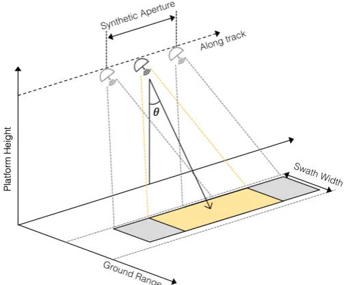
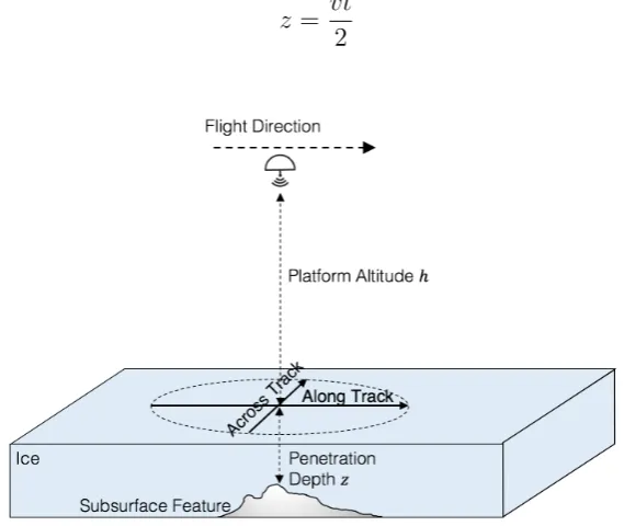
Let us consider a RS instrument is mounted on a platform flying at an altitude h0

(32)

interval (PRI). The pulse travels from the sensor to the surface, where a part of the signal is reflected or scattered. A portion of it penetrates the subsurface and is backscattered by the subsurface targets and turns back through the ice and air to the sensor. In this scenario the targets are thermal or mechanical discontinuities that implies a dielectric contrast. While sending pulses the platform is moving in the so called along-track direction and the resulting data is called radargram. A radargram is a 2D image that represents the recorded echo power for a given range position in dept as a function of time (or distance), and as a function of the instrument position in the along-track direction. Figure 2.6 shows the acquisition geometry of a RS mounted on a airborne platform. As mentioned above, the radargram can be represented in both the time or the distance (i.e., depth) domain. This conversion depends on the dielectric properties of the medium in which the radar signal propagates. In particular, the velocity of propagation can be defined as:

v = √ 1

µ0µr0r

= v√light

r

(2.15)

whereµ0 is the magnetic permeability of vacuum,µr is the material relative permeability, 0 is the dielectric permittivity of vacuum, r is the dielectric permittivity of the mate-rial. From the formula, the propagation velocity of the waves through a real material is always smaller than the speed of the wave propagating in vacuum (i.e., light speedvlight). Considering the two-way path of the wave in the air and into the material, the depth is computed according to the following equation:

z = vt

2 (2.16)

(33)

where v, and consequently r is the only parameter that relates the propagation depth z with the propagation time t. r strongly affects also the penetration capability of the RS pulse. Indeed, it affects the main factors describing the signal propagation in the medium, which are: reflection, transmission and attenuation. The reflection and transmission effects can described by the Snell’s law under the assumption of flat surface. The reflection coefficient (i.e., scattering coefficient) between two interfaces (e.g., air and ice) is defined as follows:

σs =

√ r,p− √ r,p+1 √ r,p+ √ r,p+1 2 (2.17)

where r,p and r,p+1 are the relative dielectric constants of layerpand p+ 1, respectively.

Assuming that no absorption loss is generated by the interface, the fraction of energy that is transmitted through the interface is given by the transmission coefficient τp,p+1, as

follows:

τp,p+1 = 1−σs (2.18)

An important factor that affects the signal propagation is the two-way power attenuation. The attenuation depends on the characteristics of the medium, in terms of dielectric properties (e.g., material, water content) and structure (e.g., porosity) (Fu and Daniels [2007]). It can be modeled considering an homogeneous layer according the following exponential equation:

η2_loss=e4αzz _(2.19)

where αz is the attenuation factor and z is the penetration depth in the subsurface. The attenuation factor αz is given by:

αz =ω

r µ0 2 v u u t s 1 + 00 0 2

−1 (2.20)

where ω = 2πf, µ is the magnetic permeability of the medium, and

=0r =0−i00 (2.21)

where the term represents the dielectric permittivity of the material, which is given by the product of the vacuum permittivity0 and the material relative permittivityr. Con-sidering this formulation, the attenuation is frequency dependent, it is higher at higher frequencies. This implies that at higher central frequency the penetration depth decreases.

Geometrical resolution Using a chirp signal, after the range compression, the vertical resolution of a RS mainly depends on the bandwidth Bw and is equal to:

δz =

vlight 2Bw

√

r

(34)

Overview on approaches for biophysical parameters estimation 19

Thus, the effective resolution in the subsurface depends on the material in which the wave is traveling. Usually, weighting is applied during the range compression in order to reduce the sidelobes due to the signal processing. As a result, the effective range resolution wors-ens by a factor that depends on the applied weighting function (e.g., Hanning, Hamming). It is important to note that the bandwidth of the signal is a key factor also for the gain of the system. Indeed, radar systems using chirp signals can achieve a gain equal to the range compression factor, given by:

ηz =tpBw (2.23)

In RS systems the along-track resolution after focused processing can be computed as

δalt = Vs BD

(2.24)

whereDB is the Doppler bandwidth that is:

BD = 2V_s2

h0λ

Ti (2.25)

Equation (2.8) indicates the maximum ideal integration time. In real scenarios as for spaceborne RSs, it is commonly assumed that the coherent scattering from the ground is limited by the first Fresnel zone. The diameter of the Fresnel zone DF is given by:

DF =

p

2λh0 (2.26)

According to the Fresnel zone, the effective integration time becomes:

ti,ef f = DF

Vs

(2.27)

Thus the along-track resolution calculated using the effective integration time is lower than the maximum value considering the ideal case. The number of echoes that should be processed to obtain the synthetic aperture depends on the effective integration time and the pulse repetition frequency (PRF). Such echoes are integrated to focus one resolution cell. As a consequence, the SNR of the focused signal increases by a factor that depends on the number of echoes (i.e., along-track compression factorηa).

2.2

Overview on approaches for biophysical parameters

estima-tion

(35)

2.2.1 Biophysical parameters estimation problem

The accurate estimation of biophysical parameters from remote sensing images is a chal-lenging task. From an analytical view point an estimation problem can be solved by designing the best mapping function possible that couples the parameter to be estimated (i.e., target) with a set of feature extracted from the remote sensing data. The mapping function must properly model the problem guarantying good generalization capability to minimize the overall estimation error. The main approaches presented in the remote sensing literature to solve parameter estimation problems are: i) derivation of empiri-cal data-driven relationships using empiriempiri-cal methods and ii) inversion of physiempiri-cal based theoretical models. In the following sections these approaches are presented.

2.2.2 Derivation of empirical data-driven relationships using empirical meth-ods

(36)

Overview on approaches for biophysical parameters estimation 21

Durba et al. [2007], focused on the retrieval of leaf area index from multi-angle imag-ing spectroradiometer data. SVR strategies requires the user to set internal parameters. For this reason methods for the automatic selection of this parameters are presented in Moser and Serpico [2009] and Pasolli et al. [2012]. These works exploit a functional min-imization correlated to regression errors and a multi-objective function based on a set of metrics (i.e., mean squared error and determination coefficient), respectively. More recently a multi-output SVR approach for the simultaneous estimation of different bio-physical parameters has been presented (Tuia et al. [2011]). The use of SVR demonstrated its robustness when exploited to address the estimation of biophysical parameters from microwave sensors and in particular exploiting SAR images. As an example in Pasolli et al. [2011] and Pasolli et al. [2015], the authors present regression methods based on SVR for retrieval of the SMC from Radarsat-2 data in challenging scenarios as mountains areas are for SAR data. It worth noting that, when supervised regression approaches are exploited, the capability to obtain a reliable regression function strichtly depends on the quality and quantity of the reference samples available to the learning phase of the algorithm. Small or biased training sample sets can prevent the capability of an empirical supervised estimation technique to model an accurate mapping function.

To solve this issue, semisupervised learning techniques are presented in the literature (Zhu [2010]). This approaches represent a solution to deal with low quality or small quantity training samples. Only few related works on SSL are presented in the remote sensing literature, while SSL is a deeply studied in the pattern recognition and machine learning communities. As an example, in Bazi et al. [2012] a seimisupervised regression for biophysical parameter estimation using multi-objective optimization in the field of Gaussian processes is proposed. This work aim to iteratively involve high confidence unlabeled samples in the learning phase of the regression using an iterative algorithm. At each iteration, the labels of unlabeled samples are estimated and, among them, the unlabeled samples that can improve the regression performance are selected and added to the training set. Another SSL work is presented in Camps-Valls et al. [2009]. In this work the authors presents two semi-supervised methods for the estimation of biophysical parameters in the context of SVR. These methods rely on building a graph or hypergraph Laplacian using the available labeled and unlabeled samples that are used to deform the training kernel matrix.

2.2.3 Inversion of physical based theoretical models

(37)

the electromagnetic radiation and the target variables. In the direct operational way, they simulate the response of a target object as function of: i) the target characteristics (i.e., structural, chemical and biophysical variables); and ii) the signal characteristics (i.e., wavelength, incidence angle, etc.). In the inverse operational way, the simulations can be used to represent the mapping between the measurements at the remote sensor and the target variable of interest. Due to the solid physical foundation and the wide range of applicability (in terms of both target properties and system characteristics), electromag-netic models can operate in more general scenarios also in cases where reference measures are not available. Thus, theoretical electromagnetic models with different levels of com-plexity and generality have been widely studied in the literature. When dealing with microwave emission and scattering, the most widely used model is the Integral Equa-tion Model (IEM) that can estimate backscattering coefficients in the context of different configuration of active sensors, e.g., incidence angle, polarization and central frequency (Fung et al. [1992]). Furthermore, the IEM characterizes surface soil moisture in terms of dielectric constant and surface roughness, and thus it is appropriate for soil moisture esti-mation problems from radar measurements. The electromagnetic models may have high complexity and dependence on a huge number of input parameters. This issue makes the inversion process often analytically complex. To overcome this problem, several different inversion strategies have been presented in the literature based on: i) iterative search al-gorithms, such as the Nelder-Mead and the Netwon-Rapson methods (Meroni et al. [2004] and Paloscia et al. [2008]), which iteratively use different model parameter configurations to minimize a dissimilarity measure between simulated and measured electromagnetic re-sponse of a target object, ii) look-up table matching (Darvishzadeh et al. [2008]), which searches among a set of pre-computed simulated spectra the most similar to the remote measurement and iii) regression methods (Song et al. [2009] and Duveiller et al. [2011]), which exploit a set of simulated samples (i.e., target biophysical variables and simulated electromagnetic responses).

2.3

Overview on clutter in radar sounder data

(38)

Overview on clutter in radar sounder data 23

2.3.1 Clutter problem definition

Clutter is a well known problem that affects the acquisition of RS data both from airborne and satellite platforms. Among the other sources of noise (e.g., thermal noise, speckle and sidelobes) the clutter is the most difficult to be avoided. Figure 2.7 shows the geometry of this phenomenon. The beam pulse of the RS antenna usually defines a large footprint on the ground. If the ground swath contains off-nadir topographic elements, detectable at the RS resolution, the receiver records their backscattered signals. Appearing in the radar-gram under the level of the surface, these off-nadir contributions can be mistaken with subsurface returns. The presence of strong clutter may hamper the correct interpretation of the radargrams. The strength of clutter depends on the size of the detected off-nadir target and on its slope and roughness. Moreover, the power of the received clutter return is frequency dependent. In particular, it can monotonically increase with the frequency. This is one of the driving factor in the design of the current airborne sensors that usually have central frequency in the range between 60 and 150 MHz (Peters et al. [2007], Jezek et al. [2011b]). Since at higher frequencies the ice surface appears very rough compared to the wavelength, the use of RS working at higher central frequencies (e.g., 1 GHz) can lead to unwanted clutter returns of considerable strength (Bekaert et al. [2014]). According to the RS acquisition geometry reported in Figure 2.6, clutter returns can be received from both along-track and across-track directions. Doppler filtering and SAR processing (i.e., azimuth focusing) are successful implemented to deal with along-track clutter. Azimuth focusing is able to reduce the area on the RS ground swath where the clutter is coming from. Figure 2.8 shows the reduction of the surface region that contributes to surface clutter in the along-track direction after the azimuth focusing. This reduces the clutter

(39)

Figure 2.8: Surface clutter contribution before SAR processing (light gray locus), and after focusing in azimuth direction by Doppler processing and in range by range compression (dark

gray cells). This example assumes flat topography in the absence of airplane roll.

problem to a one dimension problem. Thus, we mainly focus our interest on across-track clutter contribution because: i) SAR processing is a baseline for most of the RS systems to avoid along-track clutter, and ii) no synthetic aperture processing can be performed in the across-track direction (the illuminated points have zero Doppler shift).

The clutter issue makes the analysis of radargrams a challenging tasks. In the litera-ture, two different approaches are presented: i) techniques for clutter suppression and ii) techniques for clutter detection. In the following, suppression and detection techniques are presented.

2.3.2 Clutter suppression techniques

Clutter suppression techniques aim to eliminate or mitigate the surface clutter contribu-tion before the radargram formacontribu-tion. The capability to suppress the clutter, while the radar is acquiring the data, strictly depends on the system design. Radar systems capable to suppress the across-track clutter exploit sophisticated antenna with very directive beam pattern to illuminate a small portion of the surface or to exploit multi-channel systems, that, combining returns coming from different direction of arrivals, can underweight the antenna pattern in the expected clutter direction.

(40)

Overview on clutter in radar sounder data 25

Response (MVDR) techniques. NS provides clutter reduction at the risk of a degraded SNR, while MVDR, which represents a combination of beam steering (i.e., assuming that the clutter angles are known the antenna pattern is steered to the angle of interest) and NS, is capable to jointly minimize the power of clutter and the white noise, however it depends on prior signal-to-clutter information. Wu et al. [2011] show that a tomographic method can reject the surface clutter as well as the beam steering does. Moreover, tomo-graphic ice sounding provides good estimations of both the ice thickness and the bottom backscattering intensity. In Nielsen and Dall [2015], a multi-channel RS is used to analyze the direction of arrival (DOA) of ice sheet data collected on Antarctica. DOA estimation has been applied to data acquired with the four-channel POLARIS to improve the per-formance of surface clutter suppression techniques. The analysis of the DOA has recently recognized as a very interesting solution to address also ice thickness retrieval, icebed roughness and bed slope (Nielsen et al. [2017]). Jezek et al. [2011a] exploit a complex RS system composed of a two-way high-power transmitter and eight independent receiver channels to study the influence of surface clutter on the obscuration of the basal return at different elevations and frequencies. Moreover, using interferometric techniques the authors were able to estimate cross-track ice thicknesses and obtain strip maps of ice thickness along the flight track. Despite multi-channel RS systems have been mainly implemented for airborne platform, an attempt to suppress was envisaged on MARSIS mounting a secondary monopole antenna oriented along the nadir axis (Picardi et al. [2003]). This monopole was devoted to independently acquire the off-nadir returns. Un-fortunately, antenna calibration issues made this technical solution difficult to be applied. Also polarimetry has been presented as a possible solution in Raney [2008]. Polarimetry is based on the transmission of a circular polarized signal. Under the assumption of specular reflection, the sense of polarization can be distinguished. Nadir returns present inverted polarization, while clutter returns result in the same polarization transmitted, because of the double bounce effect. In principle, this method requires only two Rx channels (H and V) for the detection of the polarization change. The state of the art reported above demonstrate a recent growth of interest in the development of multi-channel RS systems to tackle the clutter problem.

2.3.3 Detection techniques

(41)

(42)

Chapter 3

A novel hybrid method for the

correction of the theoretical model

inversion in bio/geophysical

parameter estimation

This Chapter provides the first contribution of the thesis in the context of the estimation of biophysical parameters. In particular, it presents a novel hybrid method that aims at integrating theoretical analytical models with empirical observations. Exploiting two consecutive steps, the proposed method models and corrects deviations from reference target values when theoretical electromagnetic models are used for the inversion process. In order to estimate the deviation, in the first step two different strategies are presented: the global deviation biased (GDB) strategy, based on the assumption that the deviation is globally independent and identically distributed; and the local deviation biased (LDB) strategy, based on the assumption that the deviation is locally independent and identically distributed. Once the deviation is defined, the second step corrects the estimates obtained with the inversion of the theoretical model. The proposed hybrid method has been applied in the context of soil moisture content (SMC) estimation from microwave remotely sensed data.

3.1

Introduction

(43)

achieved by two different approaches: 1) derivation of empirical data-driven relationships; and 2) inversion of physical based theoretical electromagnetic models.

The first approach relies on the availability of labeled samples (for which reference measures are given) being used to derive an empirical mapping between remotely sensed data and target biophysical value. The empirical mapping is achieved through regression techniques, which estimate a functional relationship between a set of variables and cor-responding target values (i.e., the measurement of the parameters of interest). Different machine learning methods have been used for addressing regression problems, e.g., neu-ral networks, Gaussian Process regression, nearest neighborhood regression, kernel ridge regression, and Support Vector Regression (SVR) (Camps-Valls et al. [2006], Tuia et al. [2011], Pasolli et al. [2011]). Among several methods, the SVR has become popular due to its i) good generalization capability; ii) ability to handle problems with a small ratio between number of training samples and the size of the feature space; and iii) relatively limited computational load in the training phase (Demir and Bruzzone [2014]). The amount and the quality of the training samples are crucial to obtain accurate estimations by the use of regression algorithms. An inadequate number of training samples may cause a reduction on the estimation performance in terms of accuracy and generalization ability. However, collecting labeled samples is expensive (since generating reference measures may require significant time). Moreover, empirical observations are typically site and sensor dependent, as the reference samples are collected under specific operational conditions. This issue limits the possibility to extend the use of reference samples to different areas and different remote sensing systems since the observations remain valid only under the conditions in which reference samples have been collected (Meroni et al. [2004]).

(44)

Introduction 29

[1992]). When dealing with microwave emission and scattering, the most widely used model is the Integral Equation Model (IEM) that can estimate backscattering coefficients in the context of different configuration of active sensors, e.g., incidence angle, polarization and central frequency (Fung et al. [1992]). Furthermore, the IEM characterizes surface soil moisture in terms of dielectric constant and surface roughness, and thus appropriate for soil moisture estimation problems from radar measurements. The IEM has been further improved to consider multiple scattering effects in the Advanced IEM model (Fung [1994]) and often coupled with layered structured or three dimensional models to handle complex target such as vegetated areas (Karam et al. [1992]). The electromagnetic models may have high complexity and dependence on a huge number of input parameters. This issue makes the inversion process often analytically complex.The electromagnetic models may have high complexity and dependence on a huge number of input parameters. This issue makes the inversion process often analytically complex. Moreover, the theoretical models have two main limitations: 1) they adopt simplifying assumptions in the modeling of real phenomena, which may result in deviations from correct estimations; and 2) they neglect sensor noise, calibration errors and local propagations that may produce variability of the relations between the target variables and the features in different regions of the feature space. The first issue can be mitigated by increasing the complexity of the model, which results in reduction on the generalization ability, while the second one can be addressed by applying a statistical component to the estimation obtained by the theoretical model. However, often the results are not satisfactory. Thus, it is crucial to predict the possible deviations of the estimations when theoretical models are considered.

(45)

the simplifying assumptions) of theoretical models while keeping their generalization abil-ity and robustness due to the rigorous theoretical foundation. It is worth noting that the proposed hybrid approach requires the availability of only few labeled samples that leads to limited operational cost. In our experiments the proposed approach is applied to the estimation of soil moisture from microwave remotely sensed data. However, it is general and can be used in any other application where i) the above-mentioned limitations of the theoretical models are critical; and ii) the limited availability of field reference samples represent a strong limitation to the use of empirical observations only.

The remaining part of this Chapter is organized as follows. Section 3.2 presents the proposed hybrid method. Section 3.3 describes the data used in the experiments. Section 3.4 illustrates the experimental results. Finally, Section 3.5 draws the conclusion of this work.

3.2

Proposed hybrid method

Let us consider a remote sensing data Υ ={x1,x2, ...,xM}made up of a very large number M of samples, where xiR is the i-th sample defined as

x1_i, x2_i, ..., xd_i, i = 1, ..., M. xl_i,l = 1, ..., d, is the l−th variable of the i−th sample in Υ and d is the total number of variables (i.e., features). If ground reference samples do not exist, a possible approach to estimate the target values of each sample in Υ is to use theoretical models. Let us assume that G is a theoretical forward model, which simulates the behavior of the remotely sensed signals as a function of the target value under certain assumptions and simplifications intrinsic in its analytical formulation. The estimation problem can be defined by a functional relationship between a set of variables and corresponding estimated target values as:

y_it=G−1(xi) (3.1)

where G−1(.) represents the desired inverse mapping between the variable xi and the estimated target value y_it. Due to the simplifications and approximations intrinsic within the theoretical model formulation, the estimation is usually affected by a deviation δ(xi) from the target value yi, i.e.,

yi =G−1(xi) +δ(xi) = yit+δ(xi) (3.2) In other words the real target value of each sample can be modeled by two terms: i) the estimation derived from the inverse theoretical model function G−1_{; and ii) a deviation}

(46)

Proposed hybrid method 31

Figure 3.1: Block diagram of the proposed hybrid approach.

deviation of each unlabeled sample is crucial and depends on an availability of the prior information.

In this Chapter, we propose a hybrid approach that jointly uses the theoretical models and empirical observations (which can be related to a small number of ground reference samples) to estimate deviations associated to unlabeled samples and their final target values. Accordingly, we assume that a training set L ⊂ Υ made up of N << M pairs (xj, yj)Nj=1 is initially available, where xjR is the j-th training sample associated with the target value yjR. Note that the remaining samples in Υ (i.e., samples in Υ/L) are considered as unlabeled, i.e., the target measures of these samples are not available and should be estimated. The proposed hybrid approach consists of two consecutive steps: i) computing and modeling the deviations; and ii) estimating the final target values of unlabeled samples. Figure 3.1 shows the block scheme of the proposed hybrid approach. Each step of the approach is explained in detail in the following.

3.2.1 Computation and modeling of deviations

This first step is devoted to estimate the deviation of each unlabeled sample based on the available ground reference samples and their theoretical model estimates. To this end, initially the deviations of training samples are estimated as the differences between their correct target values (i.e., on the measurements of the parameters of interest) and the related theoretical model estimates, i.e.:

(47)

we propose two strategies that rely on two different assumptions associated to the dis-tributions of deviations in the feature space: i) the global deviation bias (GDB), which assumes that the deviations are globally independent and identically distributed (i.i.d.); and ii) the local deviation bias (LDB), which assumes that the deviations are locally i.i.d. The detailed descriptions of the proposed strategies are given in the following.

Global deviation bias (GDB)

The GDB strategy assumes that the accuracy of a theoretical model is the same within all portions of the feature space, i.e., the distribution of the deviation δ between the output and the inverse model is globally i.i.d. On the basis of this assumption, the deviation associated with each unlabeled sample xi in Υ L is considered as uniform (i.e., the same deviation value for each unlabeled sample is considered) and characterized by the average deviation values of all training samples as follows:

ˆ δ(xi) =

1

|L|

N

X

∀xj∈L

δ(xj), i= 1,2, ..., M −N (3.4)

where|L|is the total number of samples in Land ˆδ(xi) shows the estimated deviation for xi. The strategy is simple and has a low computational complexity. However, due to the simplifying assumptions intrinsic to theoretical models and the complexity of the inversion process (e.g., large number of variables and physical processes, and complex mathematical formulations), different accuracies of the theoretical model may be produced. Thus, as-signing the same amount of deviation to all unlabeled samples may reduce the estimation accuracy of parameters. It is worth noting that using this strategy implicitly assumes that the distribution of the deviation δ between the output and the inverse model is globally independent and identically distributed.

Local deviation bias (LDB)

(48)

Proposed hybrid method 33

the unlabeled sample xi in the feature space are identified. Finally, the deviation value of each unlabeled sample xi in Υ L is defined as the average deviation values of the k-nearest labeled samples located in its neighborhood, i.e.,

ˆ δ(xi) =

P

∀xj∈Lδ(xj)W(xi,xj)

P

∀xj∈LW(xi,xj)

, i= 1,2, ..., M −N (3.5)

where the function W(xi,xj) outputs 0 or 1, depending on whether or not xj is among the k-nearest neighbors of the unlabeled sample xi, i.e., W(xi,xj) = 1 if xj is one of the k nearest neighbors ofxi, and W(xi,xj) = 0 otherwise. Thus,P∀xj∈LW(xi,xj) =k.

An important issue in the LDB strategy is how to select an optimal value of the neighborhood parameter k to estimate reliable deviations. On the one hand, if the value ofk is as high as the number N of the reference samples, the results of LDB strategy are the same of those of the GDB strategy. On the other hand, selecting a smallk value may provide unreliable deviations affected by possible local noise or outliers. k is set according to a well-known rule of thumb (Mardia et al. [1982]), i.e., it is defined as the square root of the half of the total number of reference samples.

The LDB strategy avoids the unreliable estimations of deviations with the GDB strat-egy, by addressing a more realistic condition when compared to the GDB strategy. How-ever, it requires higher number of reference samples than the GDB strategy to accurately model the deviations in different portions of the feature space. Thus, in the case of availability of a small number of reference samples, the simple GDB can be preferred.

3.2.2 Estimation of the final target values

After obtaining the deviation ˆδ(xi) for each unlabeled sample xi, the final target value of that sample is obtained by the sum of theoretical model estimate and its deviation estimated by using either the GDB or LDB strategy, as:

ˆ

yi =yit+ ˆδ(xi) (3.6)

(49)

3.3

Datasets description and experimental setup

In order to assess the effectiveness of the proposed approach, several experiments were carried out on three datasets, namely Scatt, SMEX and ActPass, in the context of the estimation of SMC from microwave remotely sensed data. The three datasets have been acquired from radar instruments at different central frequencies mostly on bare soil ter-rains. The considered datasets consist of backscattering radar coefficients together with field SMC surveys. The Scatt dataset is composed of 17 soil moisture reference samples acquired in two bare fields. Remote measurements were conducted with a ground C-band scatterometer using HH and VV polarizations at 23_°and 40_°incidence angles. The terrain was characterized by an extremely variable roughness, also within the same field due to plowing practice, and a medium/dry soil moisture condition. The samples were acquired at different times, from 1998 to 2004 on an agricultural field near Matera, Italy (Mattia et al. [2003]).

The SMEX