Diffraction problems for quasilinear parabolic systems with boundary intersecting interfaces

R E S E A R C H

Open Access

Diffraction problems for quasilinear parabolic

systems with boundary intersecting

interfaces

Qi-Jian Tan

*

_{and Chao-Yi Pan}

*_{Correspondence:} [email protected] Department of Mathematics, Chengdu Normal University, Chengdu, 611130, P.R. China

Abstract

In this paper, we discuss then-dimensional diffraction problem for weakly coupled quasilinear parabolic system on a bounded domain

, where the interfaces

k (k= 1,. . .,K– 1) are allowed to intersect with the outer boundary

∂

and the coefficients of the equations are allowed to be discontinuous on the interfaces. The aim is to show the existence of solutions by approximation method. The

approximation problem is a diffraction problem with interfaces, which do not intersect with

∂

.

MSC: 35R05; 35K57; 35K65

Keywords: diffraction problem; quasilinear parabolic system; interface; approximation method

1 Introduction

Letbe a bounded domain inRnwith boundary∂(n≥), and letbe partitioned into a finite number of subdomainsk(k= , . . . ,K) separated byk, wherek,k= , . . . ,K– , are interfaces, which do not intersect with each other. For anyT> , set

QT:=×(,T], ST:=∂×[,T], := K–

k=

k, T:=×[,T].

In this paper, we consider the diffraction problem for quasilinear parabolic reaction-diffusion system in the form

⎧ ⎪ ⎪ ⎨ ⎪ ⎪ ⎩ ul

t–Ll(ul) =gl(x,t,u) ((x,t)∈QT), [ul_]

T= , [a

l

ij(x,t,ul)ulxjνi(x)]T= , ul_=ψl_{(x,t) ((x,t)∈S}

T∪ {× {}}),l= , . . . ,N,

(.)

wherex= (x, . . . ,xn),u= (u, . . . ,uN),ult:=∂ul/∂t,ulxi:=∂u

l_/∂x

i,ulx:= (ulx, . . . ,u

l xn),

Llul:= d dxi

al_ijx,t,ulul_xj+b_jlx,t,ulul_xj, l= , . . . ,N, (.)

repeated indicesiorjindicate summation from  ton,ν(x) := (ν(x), . . . ,νn(x)) is the unit normal vector to(the positive direction ofν(x) is fixed in advance), the symbol [·]T

denotes the jump of a quantity acrossT, and the coefficientsal_ij(x,t,ul_),bl

j(x,t,ul) and

gl_{(x,t,u) are allowed to be discontinuous onT. In the following, we refer to the conditions} onTin (.) as diffraction conditions.

The diffraction problems often appear in different fields of physics, ecology, and tech-nics. In some of them, the interfaces are allowed to intersect with the outer boundary∂ (see [–]). The linear diffraction problems have been treated by many researchers (see [–]). For the quasilinear parabolic and elliptic diffraction problems, when all of the in-terfaceskdo not intersect with∂, the existence and uniqueness of the solutions have been investigated in [–] by Leray-Schauder principle and the method of upper and lower solutions. In this paper, we investigate the existence of solutions of (.) when the interfaces are allowed to intersect with∂. In this case, because of the existence of the intersection ofand∂, the methods in [–] can not be extended. We shall show the existence of solutions by approximation method. The approximation problem is a diffrac-tion problem with interfaces which do not intersect with∂.

The plan of the paper is as follows. In Sect. , we give the notations, hypotheses and an example, and state the existence theorem of the solutions. Section  is devoted to the proof of the existence theorem.

2 The hypotheses, main result and example 2.1 The notations, hypotheses and main result

First, let us introduce more notations and function spaces.

For any set S, S¯ denotes its closure. The symbol⊂⊂ means that ⊂ and

dist(,∂) > . Let

{, . . . ,K–}= ∗, . . . ,K∗–

∪ _∗∗, . . . ,∗∗_K–K



,

where_k∗,k= , . . . ,K– , intersect with the outer boundary∂, andk∗∗,k= , . . . ,K–

Kdo not intersect with∂. Assume that the domainis partitioned into subdomains

∗_k, k= , . . . ,K, separated by interfaces_k∗, and partitioned into ∗∗_k,k= , . . . ,K–

K+ , separated by∗∗_k. The interface of∗_k and∗_k+ is∗_k. Then ¯ =K_k_=¯∗_k =

K–K+

k= ¯∗∗k. Set

Qk,T:=k×(,T] fork= , . . . ,K,

∗:= K–

k=

∗_k, ∗∗:= K–K

k=

∗∗_k, ∗_T:=∗×[,T], _T∗∗:=∗∗×[,T],

Q∗_k,T:=∗_k×(,T] fork= , . . . ,K,

Q∗∗_k,T:=∗∗_k×(,T] fork= , . . . ,K–K+ .

We see thatT=∗T∪∗∗T.

Cα_(Q¯

T) is the spaces of Hölder continuous inQ¯Twith exponentα∈(, ).W() and

W_,(QT) are the Hilbert spaces with scalar products (v,w)W()=

(vw+vxiwxi) dxand

(v,w)_W,  (QT)=

QT(vw+vtwt+vxiwxi) dxdt, respectively. Let

◦

W() := v∈W(),v|x∈∂= 

, W◦ , (QT) := v∈W ,

 (QT),v|(x,t)∈ST= 

For the vector functions with N-components we denote the above function spaces by Cα_(Q¯_T),W

(),W

,  (QT),

◦

W () and

◦

W,

 (QT), respectively. Moreover, we recall the following.

Definition .(see [, ]) Writeuin the split form

u=ul, [u]_al, [u]_bl

.

The vector functiong(·,u) := (g(·,u), . . . ,gN(·,u)) is said to be mixed quasimonotone in

B⊂RN with index vector (a, . . . ,aN) if for eachl= , . . . ,N, there exist nonnegative inte-gersal,bl, satisfying

al+bl=N– ,

such thatgl_(·,ul_{, [u]}

al, [u]_bl) is nondecreasing in [u]_al, and is nonincreasing in [u]_blfor all u∈B.

The following hypotheses will be used in this paper:

(H) (i) ∂andk,k= , . . . ,K– , are ofC+αfor some exponentα∈(, )and there

existθ∈(, )andρ> such that for every open ballKρcentered atx∈∂

and radiusρ≤ρ,

mes(Kρ∩)≤( –θ)mesKρ.

Assume that for eachk= , . . . ,K– ,

∗_k:ϕ_k∗(x) =  (x∈ ¯),

and

k

τ=

¯

∗_τ–_k∗= x:ϕ∗_k(x) < ∩ ¯. (.)

(ii) Assume that ⎧ ⎨ ⎩

al_ij(x,t,ul) =al_ij,k(x,t,ul), blj(x,t,ul) =blj,k(x,t,u l_),

gl_{(x,t,u) =g}l

k(x,t,u) ((x,t)∈Q∗k,T,u∈RN),k= , . . . ,K,

(.)

whereal

ij,k(x,t,ul)andblj,k(x,t,ul)are defined onQ¯T×R,gkl(x,t,u)are defined

onQ¯T×RN, and all of them are allowed to be discontinuous onT∗∗.

(iii) There exist constant vectorsM= (M_{, . . . ,M}N_{)andm= (m}_{, . . . ,m}N_),m≤M,

such that ⎧ ⎪ ⎪ ⎪ ⎪ ⎪ ⎨ ⎪ ⎪ ⎪ ⎪ ⎪ ⎩ gl

k(x,t,Ml, [M]al, [m]_bl)≤ ((x,t)∈QT), g_kl(x,t,ml, [m]al, [M]_bl)≥ ((x,t)∈QT), ml_≤ψl_(x,t)≤Ml

((x,t)∈ST∪ {× {}}),k= , . . . ,K,l= , . . . ,N,

whereal_,bl_{are all independent ofk. Let}

S:= u∈C(Q¯T) :m≤u≤M.

The vector functionsgk(·,u) = (g_k(·,u), . . . ,gN_k(·,u)),k= , . . . ,K, are mixed

quasimonotone inSwith the same index vector(a_{, . . . ,a}N_).

(iv) For eachk= , . . . ,K,k= , . . . ,K–K+ ,l= , . . . ,N,alij,k(x,t,ul),

bl_j,k(x,t,ul)∈C+α(Q¯∗∗_k,T×R)(i,j= , . . . ,n),g_kl(x,t,u)∈C+α(Q¯∗∗_k,T×S).

There exist a positive nonincreasing functionν(θ)and a positive nondecreasing functionμ(θ)forθ∈[, +∞)such that

νul

n

i=

ξ_i ≤al_ij,kx,t,ulξiξj≤μul n

i=

ξ_i, (.)

al_ij,k=al_ji,k, al_ij,kx,t,ul;bl_j,kx,t,ul≤μul, i,j= , . . . ,N. (.)

For eachl= , . . . ,N,ψl_(x,t)∈Cα₍¯ ×_[,T])∩_W,

 (×(,T))for some

domainwith⊂⊂,ψl_{(x, )∈C}+α₍¯_{k)(k= , . . . ,K), and the following}

compatibility condition on∗∗holds:

al_ijx, ,ψl(x, )ψ_xl_j(x, )νi(x)

∗∗= . (.)

Definition . A functionu is said to be a solution of (.) ifu possesses the follow-ing properties: (i) For someα∈(, ),u∈Cα_(Q¯

T)∩C,(Qk,T),k= , . . . ,K. For any given ⊂⊂ andt∈(,T), there existsα,  <α< , such thatut ∈Cα

(¯×[t,T]) and

uxj∈L(QT)∩C

α₍₍¯_{∩ ¯k)×[t,T]),k= , . . . ,K,j= , . . . ,n; (ii)usatisfies the equations}

in (.) for (x,t)∈Qk,T,k= , . . . ,K, the diffraction conditions for (x,t)∈T∩QTand the parabolic boundary conditions for (x,t)∈ST∪(× {}).

The main result in this paper is the following existence theorem.

Theorem . Let Hypothesis(H)hold.Then problem(.)has a solutionuinS.

2.2 An example

We next give an example satisfying the conditions in Hypothesis (H).

Example . In problem (.), let

n= , ϕ= (x)+ (x)– , ϕ=x+ (x)+ ,

ϕ=x– (x)– , ϕ= (x– )+ (x)– ,

∂:ϕ= , :ϕ=  (x∈I), :ϕ=  (x∈I), :ϕ= ,

whereI= [–(

√

 – )/, –] andI= [, (

√

 – )/], and let

:ϕ< , :ϕ< ,ϕ< , :ϕ< ,ϕ> ,ϕ< ,

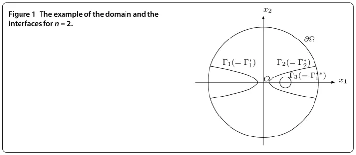
Figure 1 The example of the domain and the interfaces forn= 2.

The outer boundary of domain is a circle of radius  with the center at the origin, whereas the interface curves are two parabolas and a smaller circle of radius  (see Figure ). We see thatandintersect with∂, anddoes not.

For the coefficients of the equations and the boundary values in (.) we set

al_ijx,t,ul=

⎧ ⎨ ⎩

Al_kEl_(ul_{), i=j,}

, i=j ((x,t)∈Qk,T,u

l_{∈R),k= , , , ,i,j= , ,}

bl_jx,t,ul≡ (x,t)∈QT,ul∈R

,j= , ,

gl(x,t,u) =rl_kulf_kl(u) (x,t)∈Qk,T,u∈RN

,k= , , , ,

ψl(x,t)≡ol, l= , . . . ,N,

where

f_kl(u) =  – N

l=

δ_ll_,kul forl= , . . . ,N– , f_kN(u) =  + N–

l=

δ_lN_,kul–δ_NN_,kuN,

El(ul)∈C(R) withEl(ul)≥ν, andν,Alk,rkl,δll,k ando

l _{are all positive constants for}

k= , , , ,l,l= , . . . ,N. Then

∗_=, ∗=, ∗=, ∗=, ∗:ϕ< ,ϕ> ,

∗∗_ =, ∗∗ :ϕ< ,ϕ> , ∗∗ =.

For eachl= , . . . ,N, let

al_ij,kx,t,ul=  (x,t)∈QT,ul∈R,i= j,i,j= , ,k= , , ,

al_ii,kx,t,ul=Al_kElul (x,t)∈QT,ul∈R,i= , ,k= , ,

al_ii,x,t,ul=

⎧ ⎨ ⎩ Al

El(ul) ((x,t)∈Q∗∗,T,ul∈R),

Al_El_(ul_{) ((x,t)∈Q}∗∗

,T,ul∈R),

i= , ,

g_l(x,t,u) =

⎧ ⎨ ⎩

r_lulf_l(u) ((x,t)∈Q∗∗_,T,u∈RN),

rl

ulfl(u) ((x,t)∈Q∗∗,T,u∈RN).

We find that these functions satisfy (.) and the hypothesis (iv) of (H). Setm= (, . . . , ). Then the requirements onMin (.) become

 –δ_ll_,kMl≤, Ml≥ol,l= , . . . ,N– .

 + N–

l=

δN_l,kMl

–δ_NN_,kMN≤, MN≥oN.

It follows from these inequalities that there exist positive constant vector M, such that

mandMsatisfy (.). Furthermore, the vector functionsgk(·,u) = (g_k(·,u), . . . ,g_kN(·,u)),

k= , , , are mixed quasimonotone inSwith the same index vector (, . . . , ,N– ). The above arguments show that the conditions in Hypothesis (H) can be satisfied.

3 The proof of the existence theorem 3.1 Preliminaries

Lemma . The following statements hold true:

(i) For any givenx∈ ¯,ifϕ_k∗

(x)≤for somek

∈ {, . . . ,K– },then

ϕ_θ∗(x) <  for allθ∈ k_+ , . . . ,K– 

.

(ii) There exists a positive numberεsuch that for any givenk∈ {, . . . ,K– },if ≤θ≤k– ,then

ϕ_θ∗(x)≥ε for allx∈ y:ϕ∗k(y)≥

∩ ¯.

Proof By (.), ifx∈ ¯andϕ∗

k_(x)≤, thenx∈

k_

τ=¯∗τ. Thus for eachθ=k+, . . . ,K–,

x∈θ_τ=¯∗_τ–_θ∗. Again by (.) we getϕ_θ∗(x) < . This proves the result in (i).

For any givenk∈ {, . . . ,K– }, ifx∈ ¯andϕ_k∗(x)≥, then it follows from (i) that

ϕ∗_θ(x) >  for allθ∈ {, . . . ,k– }. Sinceϕ_θ∗∈C+α_{, there exist positive constantsε}

k,θsuch

that

ϕ_θ∗(x)≥εk,θ for allx∈ y:ϕ∗_k(y)≥∩ ¯.

Hence, the conclusion in (ii) follows from the above relation by takingε:=mink,θεk,θ.

For an arbitraryε,  <ε<ε, letsε=sε(θ) be smooth function with values between  and  such that|_dd_θsε(θ)| ≤C/εfor allθ ∈R,sε(θ) =  forθ ≤ andsε(θ) =  forθ ≥ε. Define

zε,k(x) :=

⎧ ⎪ ⎪ ⎨ ⎪ ⎪ ⎩

K–

τ= sε(ϕ∗τ(x)) (x∈ ¯),k= , K–

ϑ= [ –sε(ϕϑ∗(x))] (x∈ ¯),k=K,

K–

τ=k sε(ϕ∗τ(x)) k–

ϑ=[ –sε(ϕ∗ϑ(x))] (x∈ ¯),k= , . . . ,K– .

Lemma . zε,k(x),k= , . . . ,K,are smooth functions with values betweenand,and

possess the property

K

k=

zε,k(x) =  (x∈ ¯). (.)

Let functionsηk(x),k= , . . . ,K,be defined on¯,and let

ηε(x) =

K

k=

ηk(x)zε,k(x) (x∈ ¯). (.)

Then for any x∈ ¯,

ηε(x) = ⎧ ⎪ ⎪ ⎪ ⎪ ⎪ ⎪ ⎪ ⎪ ⎨ ⎪ ⎪ ⎪ ⎪ ⎪ ⎪ ⎪ ⎪ ⎩

η(x) ifϕ∗(x)≤,

ηK(x) ifϕK∗–(x)≥ε,

ηk(x) ifϕ_k∗_–(x)≥εandϕ_k∗(x)≤for some k∈ {, . . . ,K– },

ηk–(x)sε(ϕ_k∗_–(x)) +ηk(x)[ –sε(ϕ∗_k–(x))]

if <ϕ_k∗_–(x) <εfor some k∈ {, . . . ,K– }.

(.)

Proof Since (.) is a special case of (.) withηk(x)≡ for allk∈ {, . . . ,K}, we only prove (.).

Case . Ifϕ∗_(x)≤, then the conclusion of (i) in Lemma . implies thatϕ_k∗(x)≤ and

sε(ϕ_k∗(x)) =  for allk∈ {, . . . ,K– }. (.) yields thatzε,(x) =  andzε,k(x) =  fork≥. These, together with (.), imply thatηε(x) =η(x).

Case . Ifϕ_K∗

–(x)≥ε, then the conclusion of (ii) in Lemma . shows thatϕ

∗

k(x)≥ε andsε(ϕ_k∗(x)) =  for allk∈ {, . . . ,K– }. Hence,zε,K(x) =  andzε,k(x) =  for allk∈

{, . . . ,K– }. Again by (.) we getηε(x) =ηK(x).

Case . Ifϕ_k∗(x)≤ andϕ_k∗_–(x)≥εfor somek∈ {, . . . ,K– }, then Lemma . yields thatϕ∗_τ(x)≤,sε(ϕ_τ∗(x)) =  for allτ∈ {k, . . . ,K– }, and thatϕτ∗(x)≥ε,sε(ϕτ∗(x)) = 

for allτ∈ {, . . . ,k– }. Hence,zε,k(x) =  andzε,τ(x) =  forτ= k. Therefore,ηε(x) =

ηk(x).

Case . If  <ϕ∗_k–(x) <εfor somek∈ {, . . . ,K– }, then it follows from Lemma . thatϕ_τ∗(x) >εandsε(ϕτ∗(x)) =  for allτ∈ {, . . . ,k– }, and thatϕ∗k(x) < . Again by the conclusion of (i) in Lemma . we haveϕ_τ∗(x) <  andsε(ϕ_τ∗(x)) =  for allτ∈ {k, . . . ,K– }. Hence,zε,k(x) =  –sε(ϕ_k∗_–(x)),zε,k–(x) =sε(ϕ_k∗_–(x)) andzε,τ(x) =  forτ=k,k– .

Thus,ηε(x) =ηk–(x)sε(ϕk∗–(x)) +ηk(x)[ –sε(ϕ∗k–(x))].

3.2 The approximation problem of (1.1)

In this subsection, we construct a problem to approximate (.). For eachl= , . . . ,N, let

⎧ ⎪ ⎪ ⎨ ⎪ ⎪ ⎩

al_ijε=alijε(x,t,ul) := K

k=a l ij,k(x,t,u

l_)zε ,k(x),

bl

jε=bljε(x,t,ul) := K

k=blj,k(x,t,ul)zε,k(x),

gεl=glε(x,t,u) := K

k=g l

k(x,t,u)zε,k(x) ((x,t)∈QT).

It follows from hypothesis (iv) of (H), (.) and (.) that al_ijε(x,t,ul), bljε(x,t,ul) are in C+α_(Q¯∗∗

k,T×R) (i,j= , . . . ,n),gεl(x,t,u) is inC+ α_(Q¯∗∗

k,T×S) (k= , . . . ,K–K+ ), the vector functiongε(·,u) = (g

ε(·,u), . . . ,gεN(·,u)) is mixed quasimonotone inSwith

in-dex vector (a_{, . . . ,a}N_{), and}

νul

n

i=

ξ_i ≤alijε

x,t,ulξiξj≤μul n

i=

ξ_i, (.)

al_ijε=aljiε, alijε

x,t,ul;bl_jε

x,t,ul≤μul, i,j= , . . . ,n. (.)

We note that the functionsal

ijε(x,t,ul),bljε(x,t,ul) andgεl(x,t,u) are continuous onT∗, and are allowed to be discontinuous on_T∗∗.

For eachk= , . . . ,K–K, there exists∗τ_k such that∗∗k ⊂∗τ_k. Take two subdo-mainsBk,, Bk,satisfying_k∗∗ ⊂Bk,⊂⊂Bk,⊂⊂∗τ_k. Letλk=λk(x) be an arbi-trary smooth function taking values in [, ] such thatλk=  forx∈/∗τ_k andλk=  for

x∈Bk,. Set

ψ_εl =ψ_εl(x,t)

:=

|x–y|≤ε

ω|x–y|

 – K–K

k=

λk(y)

ψl(y,t) dy+ K–K

k=

λk(x)ψl(x,t) (.)

with a sufficiently smooth nonnegative averaging kernelω(|ξ|) that is equal to zero for

|ξ| ≥ and is such that_|ξ≤ω(ξ) dξ = . Then from the hypothesis (iv) of (H) and [, Chapter II] we know that for eachl= , . . . ,N,ψ_εl(x,t) is inCα_(Q¯

T)∩W,(QT),ψεl(x, )

is inC+α₍¯∗∗

k) (k= , . . . ,K–K+ ),ψεl→ψl inCα(Q¯T) andψεl→ψlinW

,  (QT). Thus,

ψ_εl(x,t)_Cα(Q¯T)+ψ

l

ε_W,

 (QT)≤μ, (.)

whereμis a positive constant, independent ofε. Furthermore, (.), (.) and (.) show that for small enoughε,

al_ijε

x,t,ul=al_ij,τ_k

x,t,ul,

ψ_εl(x,t) =ψl(x,t) (x,t)∈Bk,×[,T]

,k= , . . . ,K–K.

These, together with (.), imply that

aijε

x, ,ψ_εl(x, )ψ_εl_x

j(x, )νi

∗∗= . (.)

For any givenε,  <ε<ε, consider the approximation diffraction problem of (.)

⎧ ⎪ ⎪ ⎨ ⎪ ⎪ ⎩ ul

t–Llε(ul) =gεl(x,t,u) ((x,t)∈QT), [ul]∗∗_T = , [alijε(x,t,ul)ulxjνi(x)]∗∗T = , ul=ψ_εl(x,t) ((x,t)∈ST∪ {× {}}),l= , . . . ,N,

where

Llε

ul:= d dxi

al_ijε

x,t,ulul_xj+bl_jε

x,t,ulul_xj.

We note that the interfaces in (.) are_k∗∗(k= , . . . ,K–K) which do not intersect with

∂. In view of (.), the compatibility condition on∗∗holds.

Proposition . Problem(.)has a unique piecewise classical solutionuε=uε(x,t)in

Spossessing the following properties:

uε∈Cα(Q¯T), uεt∈Cα,α/(Q¯T), uεxj∈C

α,α/_Q¯∗∗

k,T α∈(, )

,

uεxjt∈L

_(Q

T), uεxixj∈C

Q∗∗_k,T, k= , . . . ,K–K+ .

(.)

Proof Problem (.) is a special case of [, problem (.)] without time delays. Formulas (.) and (.) show thatu˜=M,uˆ=mare a pair of bounded and coupled weak upper and lower solutions of (.) in the sense of [, Definition .]. We find that the conditions of [, Theorem .] are all fulfilled. Then from [, Theorem .], we obtain that problem (.) has a unique piecewise classical solutionuε=uε(x,t) inSpossessing the properties

in (.).

3.3 The uniform estimates ofuε

In the following discussion, letKρbe an arbitrary open ball of radiusρwith center atx_, and letQρbe an arbitrary cylinder of the formKρ×[t_–ρ_,t_].

For each l= , . . . ,N, consider the equality _tt



[u

l

εt –Llε(uεl)]ηldxdt= t

t

g

l

ε(x,t, uε)ηl_{dxdtfor any functionη}l_=ηl_{(x,t) from W}◦ ,

 (QT) withess supQT|η

l_{|<∞ and for}

anyt,tfrom [,T]. In view ofuε∈S, it follows from (.), (.), (.) and the formula of

integration by parts that

ulεηldx

t t + t t

–ulεηlt+alijε

x,t,ulε

ulεxjη

l xi

dxdt

= t t

–bl_jεx,t,ul_εul_εxj+g_εl(x,t,uε)

ηldxdt (.)

≤C t t _ul

εx+ ηldxdt. (.)

Similarly, for anyφl∈W◦ () and for everyt∈[,T] we get

al_ijε

x,t,ulε

ulεxjφ

l xidx=

–ulεt–bljε

x,t,ulε

ulεxj+g

l

ε(x,t,uε)

φldxdt. (.)

Lemma . There exist constants α ( < α < ) and C depending only on M (:=

max(|M|,|m|)),ρ,θ,α,ν(M),μ(M)andμ,independent ofε,such that

ulε_Cα,α/_(Q¯_T)≤C, (.)

ulεxL_(Q

Proof (.) follows from (.), (.), (.), (.) and [, Chapter V, Theorem . and Remark .]. Settingηl=ul

ε–ψεl in (.) and using Cauchy’s inequality, we can obtain

(.).

Lemma . For any given k_∈ {, . . . ,K},let D⊂⊂∗_k

and t

_{∈(,T).Then there exist} positive constantsα( <α< )and C(d,t)depending only on d (:=dist(D,∂∗_k

)),t

and the parameters M,ρ,θ,α,ν(M),μ(M)andμ,independent ofε,such that for

any∗∗_ksatisfying D∩∗∗_k=∅,

ulεxjCα((D∩∗∗_k)×[t,T])≤C

d_,t, j= , . . . ,n,l= , . . . ,N, (.)

ul_εtCα(D¯×[t,T])≤C

d_,t, l= , . . . ,N. (.)

For any given k∈ {, . . . ,K},let⊂⊂k and t∈(,T).Then there exist positive

con-stants α ( <α< ) and C(d,t)depending only on d (:=dist(,∂k)),tand the

parameters M,ρ,θ,α,ν((M)),μ(M)andμ,such that

ulεC+α,+α/(¯×[t,T])≤C

d,t, l= , . . . ,N. (.)

Proof Choose a subdomainBsatisfyingD⊂⊂B⊂⊂∗_k

. (.) and (.) show that for

small enoughε,

⎧ ⎪ ⎪ ⎪ ⎨ ⎪ ⎪ ⎪ ⎩ al

ijε(x,t,ul) =alij,k_(x,t,u l_),

bl

jε(x,t,ul) =blj,k_(x,t,u l_),

gl

ε(x,t,u) =g_kl

(x,t,u) ((x,t)∈B×(,T]),l= , . . . ,N.

(.)

Then the same proofs as those of [, formulas (.) and (.)] give (.) and (.). If ⊂⊂k, then⊂⊂∗_k

∩

∗∗_kfor somek∈ {, . . . ,K},k∈ {, . . . ,K–K+ }. Hence, the conclusion in (.) follows from (.), (.), (.) and the same argument as that

for [, formula (.)].

In the rest of this subsection, letk_be an arbitrary fixed number in{, . . . ,K– }, and let

D⊂⊂be an arbitrary fixed subdomain satisfyingD∩_k∗

 =∅,

¯ D∩(_k∗

–∪

∗

k_+) =

∅andD¯∩∗∗=∅. We next investigate the uniform estimates in the neighborhood of

∗_k

∩ ¯D. Letx

_{be any point of}∗

k_∩ ¯D. [, Chapter , Section ] and [] show that there exists a ballKρwith center atx_{such that we can straighten}∗

k_∩Kρout by introducing a local coordinate systemy=y(x). Our assumptions concerningimply that we can divide ∗

k_∩ ¯D into a finite number of pieces and to introduce for each of them coordinatesy. Since the investigations in the rest of this subsection are local properties, we can assume without loss of generality that the interface_k∗

lies in the planexn= . Then by (.), when

(x,t)∈D×[,T] the coefficients of problem (.) can be represented in the form

⎧ ⎪ ⎪ ⎪ ⎨ ⎪ ⎪ ⎪ ⎩ al

ijε(x,t,ul) =al_ij,k

(x,t,u

l_{)sε(xn) +a}l

ij,k_+(x,t,u

l_{)[ –sε(xn)],}

bl

jε(x,t,ul) =blj,k_(x,t,u l_)sε(x

n) +bl_j,k

+(x,t,u

l_{)[ –sε(x} n)],

gεl(x,t,u) =g_kl

(x,t,u)sε(xn) +g

l

k+(x,t,u)[ –sε(xn)], l= , . . . ,N,

and the diffraction conditions on∗_Tin problem (.) can be represented in the form

ul∗

T= ,

al_njx,t,ulul_xj∗

T= , l= , . . . ,N. (.)

Lemma . Let t∈(,T).Then there exist positive constantsα( <α< )and C(d,t)

depending only on d_(:=min{dist(D,∂),dist(D,_k∗

–∪

∗

k+),dist(D,

∗∗_{)}),t,and the} parameters M,ρ,θ,α,ν(M),μ(M)andμ,independent ofε,such that

ulεxsCα_(D¯_×[t,T])≤C

d_,t, s= , . . . ,n– , (.)

_εl_,n

Cα(D¯×[t,T])≤C

d_,t, _εl_,n:=al_njε

x,t,ulε

ulεxj, (.) ulεtCα(D¯×[t,T])≤C

d_,t, l= , . . . ,N. (.)

Proof It follows from (.) and Hypothesis (H) that

∂alijε(x,t,ul)

∂xs

;∂a l ijε

∂t ;

∂al_ijε

∂ul

+∂b

l

jε(x,t,ul)

∂xs ;∂b

l jε

∂t ;

∂bl_jε

∂ul

+∂g

l

ε(x,t,u)

∂xs ;∂g

l

ε

∂t ;

∂gl

ε

∂ul

≤C (x,t)∈ ¯D×[,T],u∈S

,s= , . . . ,n– ,l,l= , . . . ,N, (.)

and from the equations in (.) that

_dd_xnal_njεx,t,ul_εul_εxj≤C

ul_εt+ n–

s= n

j=

ul_εxjxs+ul_εx+ 

(x,t)∈ ¯D×[,T]

,l= , . . . ,N. (.)

Then using (.), (.), (.), (.) and (.), we can prove (.)-(.) by a slight modification of the proofs of [, formulas (.) and (.)]. The detailed proofs are

omit-ted.

3.4 The proof of Theorem 2.1

From estimates (.), (.) and the Arzela-Ascoli theorem it follows that we can find a subsequence (we retain the same notation for it){uε}such that{uε}converges inC(Q¯T) to

uand{uεxj}converges weakly inL(QT) touxj for eachj= , . . . ,n. Thenu∈C

α_(Q¯_{T) and}

u_xj∈L_(Q

T). Furthermore, the parabolic boundary conditions foruεin (.) imply that usatisfies the parabolic boundary conditions in (.).

For any givenk∈ {, . . . ,K}, and for any⊂⊂k,t∈(,T), (.) yields that there exists a subsequence{uε}(denoted by{uε} still) such that{uε}converges in C,(¯×

[t,T]) tou. By lettingε→, from (.) and the equationsul

εt–Llε(ulε) =gεl(x,t,uε) in

(.) we get that

ul_t–Llul=gl(x,t,u) (x,t)∈×t,T,l= , . . . ,N.

Sinceandtare arbitrary, thenusatisfies the equations in (.) for (x,t)∈Qk,T. For any givenk∈ {, . . . ,K}and for anyD⊂⊂∗_k

,t

_{∈(,T), we see from (.), (.)}

and for any∗∗_ksatisfyingD∩_k∗∗=∅,{uεxj}converges inC((D∩∗∗k)×[t,T]) touxj,

and{uεt}converges inC(D¯×[t,T]) tout. Hence

uxj∈C α_D

∩∗∗_k×t,T, ut∈Cα

_¯ D×

t,T. (.)

By lettingε→ we conclude from (.) and the diffraction conditions on_T∗∗foruεin

(.) that

ul∗∗

T∩QT= ,

al_ijx,t,ulul_xjνi(x)∗∗

T∩QT= , l= , . . . ,N. (.)

For any givenk_∈ {, . . . ,K– }andD⊂⊂satisfyingD∩∗_k

=∅,

¯ D∩(_k∗

–∪

∗_k

+) =∅and

¯

D∩∗∗=∅, the estimates (.)-(.) imply that for any givent∈(,T) there exists a subsequence{uε}(denoted by{uε}still) such that for eachs= , . . . ,n– , l= , . . . ,N,

ulεxs→u

l

xs, u

l

εt→ult, εl,n=alnjε

x,t,ulε

ulεxj→

l _inCD¯

×

t,T.

(.)

Then

ul_xs,ul_t,l∈Cα_D¯

×

t,T. (.)

We next show thatl=al

nj(x,t,ul)ulxj. For anyη=η(x,t)∈L

_(D

×(t,T)),

T

t

D

al_njεx,t,ul_εul_εxj–al_njx,t,ulul_xjηdxdt

= T t D

al_njεx,t,ul_ε–al_njεx,t,ulul_εx jηdxdt

+ T t D al_njε

x,t,ul–al_njx,t,ululεxjηdxdt

+

T

t

D

al_njx,t,ululεxj–u

l xj

ηdxdt

:=I_εl_,+I_εl_,+I_εl_,.

By (.), (.), we get

Iεl,≤Culε–ul

η_L_(D

×(t,T))u

l

εxjL_(D ×(t,T))

≤Cul_ε–ulη_L_(D

×(t,T))→ asε→,

and by (.), (.),

Il

ε, =

T

t

D∩{x|≤xn≤ε}

al nj,k_

x,t,ul_–al nj,k_+

x,t,ul_sε(x

n)ulεxjηdxdt

≤ CulεxjL_(D ×(,T))

T

t

D∩{x|≤xn≤ε}

≤ C

T

t

D∩{x|≤xn≤ε}

ηdxdt /

→ asε→.

Since{uεxj}converges weakly inL

_{(QT) tou}

xj for eachj= , . . . ,n, thenI

l

ε,→ asε→. Hence,_εl_,n=al_njε(x,t,ulε)ulεxjconverges weakly inL

_(D

×(t,T)) toalnj(x,t,ul)ulxjfor each j= , . . . ,n. This, together with (.), implies that

l=al_njx,t,ulul_xj∈Cα_D¯

×

t,T, (.)

andusatisfies the diffraction conditions on∗_T∩QTin (.).

In view of (.)usatisfies the diffraction conditions onT∩QTin (.). Furthermore, (.), (.) and (.) imply that for anyk∈ {, . . . ,K},⊂⊂,

uxj∈C

α_∩

k

×t,T, ut∈Cα

_¯

×t,T, j= , . . . ,n

for someα∈(, ). Therefore,uis a solution of (.). This completes the proof of Theo-rem ..

Competing interests

The authors declare that they have no competing interests.

Authors’ contributions

All authors read and approved the final manuscript.

Acknowledgements

Dedicated to Professor Hari M Srivastava.

The authors would like to thank the reviewers and the editors for their valuable suggestions and comments. The work was supported by the research fund of Department of Education of Sichuan Province (10ZC127) and the research fund of Chengdu Normal University (CSYXM12-06).

Received: 19 January 2013 Accepted: 9 April 2013 Published: 22 April 2013 References

1. Ladyzenskaya, OA, Solonnikov, VA, Ural’ceva, NN: Linear and Quasilinear Equations of Parabolic Type. Am. Math. Soc., Providence (1968)

2. Ladyzenskaya, OA, Ural’ceva, NN: Linear and Quasilinear Elliptic Equations. Academic Press, New York (1968) 3. Ladyzenskaya, OA, Ryvkind, VJ, Ural’ceva, NN: Solvability of diffraction problems in the classical sense. Tr. Mat. Inst.

Steklova92, 116-146 (1966) (in Russian)

4. Yi, FH: Global classical solution of Muskat free boundary problem. J. Math. Anal. Appl.288, 442-461 (2003) 5. Druet, PE: Global Lipschitz continuity for elliptic transmission problems with a boundary intersecting interface.

Weierstrass Institute for Applied Analysis and Stochastics, WIAS Preprint No. 1571 (2010)

6. Kamynin, LI: On the linear Verigin problem. Dokl. Akad. Nauk SSSR150, 1210-1213 (1963) (in Russian)

7. Kamynin, LI: The method of heat potentials for a parabolic equation with discontinuous coefficients. Sib. Mat. Zh.4, 1071-1105 (1963) (in Russian)

8. Chen, Z, Zou, Z: Finite element methods and their convergence for elliptic and parabolic interface problems. Numer. Math.79, 175-202 (1998)

9. Huang, J, Zou, J: Some new a priori estimates for second-order elliptic and parabolic interface problems. J. Differ. Equ. 184, 570-586 (2002)

10. Evans, LC: A free boundary problem: the flow of two immiscible fluids in a one-dimmensional porous medium. I. Indiana Univ. Math. J.26, 914-932 (1977)

11. Rivkind, V, Ural’tseva, N: Classical solvability and linear schemas for the approximated solutions of the diffraction problem for quasilinear elliptic and parabolic equations. Mat. Zametki3, 69-111 (1972) (in Russian)

12. Boyadjiev, G, Kutev, N: Diffraction problems for quasilinear reaction-diffusion systems. Nonlinear Anal.55, 905-926 (2003)

13. Tan, QJ: Systems of quasilinear parabolic equations with discontinuous coefficients and continuous delays. Adv. Differ. Equ.2011, Article ID 925173 (2011). doi:10.1155/2011/925173

14. Tan, QJ, Leng, ZJ: The method of upper and lower solutions for diffraction problems of quasilinear elliptic reaction-diffusion systems. J. Math. Anal. Appl.380, 363-376 (2011)

doi:10.1186/1687-2770-2013-99