Turkish Journal of Fisheries and Aquatic Sciences 13: 261-270 (2013)
www.trjfas.org ISSN 1303-2712 DOI: 10.4194/1303-2712-v13_2_08
© Published by Central Fisheries Research Institute (CFRI) Trabzon, Turkey in cooperation with Japan International Cooperation Agency (JICA), Japan
Testing the Sensitivity of the Length-Converted Catch Method Using the
Bigeye Tuna
Thunnus obesus
(Scombridae) Population Parameters
Introduction
The total mortality (Z) of fish, which is composed of fishing mortality and natural mortality, is an important biological parameter for conducting stock assessments. The parameter Z is used to estimate fishing mortality by directly subtracting natural mortality from Z. Fishing mortality is generally used to determine stock status, such as overfishing, by comparing with biological reference points such as F0.1, F40%, F30%, and Fmax. However,
natural mortality is often assumed to be constant and is usually either estimated empirically (Pauly, 1980; Hoenig et al., 1987; Chen and Watanabe, 1989) or evaluated by experts (Nishida and Shono, 2006). Thus, the accuracy of Z estimates affects the determination of stock status remarkably.
The parameter Z is generally estimated using the length-converted catch method (LCCM) (Pauly, 1983), and a full year’s length data are often needed in the calculation of this method under the assumption of an equilibrium state. Several studies have used the LCCM to investigate the impacts of growth curves on the estimates of Z, whichcan be overestimated due to seasonal growth patterns (Pauly, 1995; Sparre, 1990); therefore, growth variation and the accuracy of the
growth curves influence Z markedly (Hampton and Majkowski, 1987; Castro and Erzini, 1988).
The LCCM assumes that fish dynamics are characterized by an equilibrium state. However, an equilibrium state may be impossible to attain, especially for exploited fish stocks, which usually suffer various fishing levels due to the variation in the number of fishing boats, fishery management styles, and other factors. Fishing levels also affect both Z and recruitment levels. The sample size and length interval size adopted in the LCCM also create uncertainty in the estimation of Z. Therefore, determining a smaller sample size in order to improve the accuracy Z is important for yielding cost-effective data.
In the present study, a Monte Carlo simulation method is applied using the LCCM to assess how these factors influence the estimation of Z. This method is used to generate length frequency data based on known parameters, while simulated data are applied in the LCCM to estimate Z. These Z estimates are then compared with the known Z values to determine their accuracy for each scenario. This convenient approach allows researchers to examine whether a sampling strategy influences the estimated parameters before they complete the sample design
Chia-Lung Shih
1,*
1
Institute of Oceanography, College of Science, National Taiwan University, Institute of Oceanography, National Taiwan University, 1, Section 4, Roosevelt Road, Daan District, Taipei, Taiwan.
* Corresponding Author: Tel.: +86.912 768647; Fax: +86.912 768647; E-mail: [email protected]
Received 25 September 2012 Accepted 10 April 2013
Abstract
The present study investigates how sample size, length interval size, recruitment variation, and mortality over time influence total mortality, which is estimated by applying the length-converted catch method to the bigeye tuna (Thunnus obesus) population. Given the assumption of fish dynamics under an equilibrium state, an increasing sample size and decreasing length interval size can raise the accuracy of total mortality estimates, with a sample size of 3000 individuals and length class interval of 5 cm generally producing the most accurate estimates. When fish dynamics follow a non-equilibrium state, randomly varied recruitment does not affect the estimation of total mortality. However, recruitment that varies with increasing or decreasing trends would affect total mortality remarkably. Therefore, total mortality that varies by time influences estimated total mortality, and in this situation, fish stocks that undergo stable total mortality for four successive years could produce an accurate total mortality figure. Finally, we suggest that the non-equilibrium state of fish dynamics should be considered before applying the length-converted catch method to estimate Z.
and select the optimal approach to analyze the resultant data. This method has also been used to determine the optimal sample size for estimating growth parameters accurately using length frequency analysis (Erzini, 1990).
This study uses the case study of bigeye tuna (Thunnus obesus), a species that has economic and ecological importance and that has been exploited since the 1950s (Okamoto and Miyabe, 1999). Many researchers have studied this species in order to protect stocks, and thus biological and fishery parameters (such as growth parameters, mortality, and gear selectivity) have been investigated using various methods. Such detailed information about this species enables us to simulate its stock dynamics reliably. According to the stock assessments of this species, recruitment levels greatly vary over time, while a time series of fishing mortality is also variable (Nishida and Shono, 2006; Langley et al., 2008). In addition, because this species has a long lifespan (Farley et al., 2006), estimating Z using the LCCM might be sensitive to the non-equilibrium state. The LCCM have been applied in this species (Zhu et al., 2009) and thus, we should understand the sensitivity of the LCCM when estimating bigeye tuna parameters.
This study investigates how sample size and length class affect Z estimates and what levels of recruitment deviation and mortality changes over time influence Z. It is anticipated that the results will provide information on in which situations the LCCM could be applied in order to obtain more accurate Z
estimates.
Materials and Methods
As noted in the Introduction, the Monte Carlo simulation method was used to generate length data under various fish dynamics scenarios. The parameters for bigeye tuna used in these simulations were assumed to be known, including growth parameters, recruitment variation, total mortality, and gear selectivity.
First, catch-at-age data were generated based on the known age structure of the population caught by a longline fishery. Catch-at-age data were used to randomly generate the corresponding length-at-age distributions based on the known mean length-at-age. Then, length data were converted into length frequency data by length interval size, and these length frequency data were used to estimate Z using the LCCM. The above steps were replicated 500 times. Finally, the mean and standard deviation (SD) of the 500 replicates of the simulated Z values were estimated to assess their accuracy relative to the estimates. The details of this process are described below.
Simulated Population Dynamics of Bigeye Tuna
The age composition for the bigeye tuna
population was simulated using the following dynamics equation:
1 exp ....(1)
i i
N N Z
where Ni is the population at age i and Ni+1 is the
number of survivors at age i+1.
Z was assumed to be constant for all age classes, and the maximum age of bigeye tuna was assumed to be eight years. Although the maximum recorded age of this species is about 16 years (Farley et al., 2006), the proportion of the sample larger than eight years old was small in both the simulations of this study (<2%) and in actual catches (Farley et al., 2006). Moreover, fishing behavior was assumed to operate in the middle of the month, and thus the dynamics by month were represented by
1, , exp ....(2)
24 12
m i m i
Z Z
N N
where Nm,i is the abundance of population at age
i in month m.
Gear Selectivity
The length data of bigeye tuna used to estimate
Z are usually collected from longline fisheries (Zhu et al., 2011). Other fisheries, such as purse seines, also often fish this stock as a bycatch. However, for simplicity, only longline fisheries were considered to exploit this stock in the presented simulations. The gear selectivity of longline fisheries is usually thought to follow a logistical curve (Nishida and Shono, 2006). Thus, gear selectivity was assumed to be 0.5 at age one year and 1.0 for ages older than one year. Catch-at-age data were then estimated from the dynamics equation (2) using gear selectivity. The simulated sample size was assumed to be collected for each month uniformly.
Length-at-Age
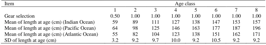
In this process, the simulated catch-at-age was converted into the corresponding length-at-age. The birthday of bigeye tuna was assumed to be January 1. Length data were assumed to have a normal distribution with an SD for each age. Length-at-age data were then generated based on the corresponding exact age derived from the von Bertalanffy growth parameters and length-at-age SD. The von Bertalanffy growth parameters of bigeye tuna from the three oceans were L∞=169 cm, k=0.32 year-1, and t0=-0.34
year (Stéquert and Conand, 2004) for the Indian Ocean, L∞=229 cm, k=0.23 year-1, and t0=-0.43 years
(Lehodey et al., 1999) for the Pacific Ocean, and
L∞=217 cm, k=0.18 year-1, and t0=-0.61 years for the
al., 2006), which were used to approximate the estimates, and was assumed to be equal for the three populations. The length-at-age mean and SD are shown in Table 1.
LCCM Formulation
In the LCCM (Pauly, 1983), length frequency was converted into relative age frequency using the growth parameters L∞ and k. The equation to estimate
Z was as follows: where
i
L
t
is the
11
ln
/
...(3)
2
i i i i
L L
L L i
t
t
C
dt
a
Z
relative age for the ith length class,
1
i i
L L
C
is the catch between the ith and i+1th length classes, and dtiis the time needed for fish to grow through the length class.
Z can be estimated using a linear relationship. However, some small length data may be younger than the age that was fully recruited into the fishery and the sample sizes in some ith length classes too small, which may adversely affect the estimation of Z. The criteria used to choose the relative age range for estimating Z were between the relative age with the
value next to the highest
1
ln /
i i
L L i
C dt
after the
relative age of 2.5 years and the relative age with a
value of
1
ln
/
i i
L L i
C
dt
greater than or equal to 3.5.
Estimation of Accuracy and Precision
The proportion error was used to represent the accuracy of the simulated Z as follows:
% 100%
i k...(4)
i k
P
P
E
P
where Ei% is the proportion error of the
simulated Z for case i, Pi is the mean of the 500
replicates of the simulated Z for case i, and Pk is the
kth true level of Z.
Further, the coefficient of variance (CV) was used to represent the precision of the estimates as follows:
/ ...(5)
i i i
CV
SD P
where SDi is the SD of the 500 replicates of the
simulated Z for case i.
Sensitivity Analysis
The following nine scenarios were considered in the presented sensitivity analysis:
S0: This is the base case (an equilibrium state) in which fish dynamics were assumed to suffer from constant mortality for 10 successive years as well as undergoing constant recruitment. Five levels of initial
Z – 0.40, 0.60, 0.80, 1.00, and 1.20 year-1 – were considered to simulate fish dynamics. Five sample sizes, namely 500, 1000, 3000, 5000, and 10,000 individuals, were then used to generate length data, while five length interval sizes, 1, 5, 10, 15, and 20 cm, were considered to convert these length data. Note that only the most optimal sample and length interval sizes derived from the results of S0 were adopted in the following scenarios:
S1: The same as S0, but annual recruitment variation was assumed to vary randomly:
S1-2: Varying by 5%. S1-3: Varying by 10%. S1-4: Varying by 20%. S1-5: Varying by 30%.
S2: The same as S1, but annual recruitment variation was assumed to have an increasing trend:
S2-1: Increasing by 5%. S2-2: Increasing by 10%. S2-3: Increasing by 15%. S2-4: Increasing by 20%.
S3: The same as S1, but annual recruitment variation was assumed to have a decreasing trend:
S3-1: Decreasing by 5%. S3-2: Decreasing by 10%. S3-3: Decreasing by 15%. S3-4: Decreasing by 20%.
S4: The same as S1, but total annual mortality was assumed to have an increasing trend:
S4-1: Total annual mortality increased slightly by 0.40, 0.45, 0.50, 0.55, 0.60, 0.65, 0.70, 0.75, 0.80, and 0.85 year-1.
S4-2: Total annual mortality increased largely by 0.40, 0.50, 0.60, 0.70, 0.80, 0.90, 1.00, 1.10, 1.20, and 1.30 year-1.
S5: The same as S1, but total annual mortality was assumed to have a decreasing trend:
S5-1: Total annual mortality decreased slightly by 0.85, 0.80, 0.75, 0.70, 0.65, 0.60, 0.55, 0.50, 0.45,
Table 1. The assumed true parameters of gear selectivity, and mean and standard deviation (SD) length-at-age used in the simulations
Item Age class
1 2 3 4 5 6 7 8
and 0.40 year-1.
S5-2: Total annual mortality decreased largely by 1.30, 1.20, 1.10, 1.00, 0.90, 0.80, 0.70, 0.60, 0.50, and 0.40 year-1.
S6: The same as S1, but total annual mortality increased largely and then stabilized:
S6-1: 0.40, 0.60, 0.80, 1.00, 1.20, 1.40, 1.40, 1.40, 1.40, and 1.40 year-1.
S6-2: 0.40, 0.40, 0.60, 0.80, 1.00, 1.20, 1.40, 1.40, 1.40, and 1.40 year-1.
S6-3: 0.40, 0.40, 0.40, 0.60, 0.80, 1.00, 1.20, 1.40, 1.40, and 1.40 year-1.
S6-4: 0.40, 0.40, 0.40, 0.40, 0.60, 0.80, 1.00, 1.20, 1.40, and 1.40 year-1.
S7: The same as S1, but total annual mortality increased slightly and then stabilized:
S7-1: 0.40, 0.45, 0.50, 0.55, 0.60, 0.65, 0.65, 0.65, 0.65, and 0.65 year-1.
S7-2: 0.40, 0.40, 0.45, 0.50, 0.55, 0.60, 0.65,
0.65, 0.65, and 0.65 year-1.
S7-3: 0.40, 0.40, 0.40, 0.45, 0.50, 0.55, 0.60, 0.65, 0.65, and 0.65 year-1.
S7-4: 0.40, 0.40, 0.40, 0.40, 0.45, 0.50, 0.55, 0.60, 0.65, and 0.65 year-1.
S8: The same as S1, but total annual mortality was stable for the first five years and then increased gradually:
S8-1: Increased largely: 0.40, 0.40, 0.40, 0.40, 0.40, 0.50, 0.60, 0.70, 0.80, and 0.90 year-1.
S8-2: Increased slightly: 0.40, 0.40, 0.40, 0.40, 0.40, 0.45, 0.50, 0.55, 0.60, and 0.65 year-1.
Results
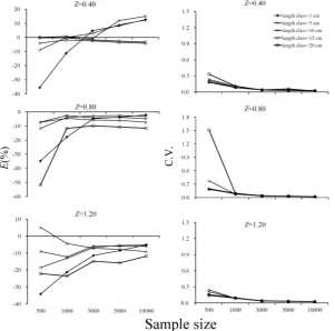
The results of the simulated Z for the bigeye tuna populations of all three oceans showed similar trends in S0 (Figures 1-1, 1-2, 1-3), and those of the
Figure 1-2. Proportion error (E(%)) and coefficients of variation (C.V) for the simulated total mortality (Z) for bigeye tuna in the Pacific Ocean among all cases generated by the simulations in S0.
Atlantic and Pacific Oceans only showed the cases of
Z=0.40, 0.80, and 1.20 year-1. The factors of sample size, length interval size, and initial Z affected the accuracy of the simulated Z remarkably (Figure 1-1). Increasing the sample size improved the accuracy of the simulated Z except for the case of Z=0.40 year-1. The simulated Z (in the case of Z=0.40 year-1) was underestimated for small sample sizes (e.g. 500 individuals), accuracy was optimized at sample sizes of up to 1000 individuals, and then Z became overestimated at sample sizes over 3000 individuals. Moreover, using smaller length interval sizes (1 cm and 5 cm) tended to yield more accurate estimates. By contrast, for a small sample size (i.e. 500 individuals), using larger length interval sizes produced a higher degree of accuracy.
Further, increasing sample size above 1000 individuals raised the precision of the estimates and maintained them at a high level (Figure 1-1). However, for a small sample size (i.e. 500 individuals), length class interval affected precision remarkably. Larger length interval sizes (15 cm and 20 cm) also produced lower precision. In conclusion, for a sample size of 3000 individuals and length interval size of 5 cm, the accuracy and precision of estimates was high; therefore, these values were adopted in the subsequent scenario simulations (S1– S8). Moreover, only the bigeye tuna population of the Indian Ocean was considered in the further analysis.
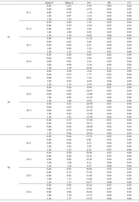
In the simulations with randomly varied recruitment (S1), the level of variation did not seem to affect the accuracy and precision of estimates even at large levels (i.e. 30%) (Table 2). However, in the simulations of fish dynamics with decreasing or increasing recruitment trends by time series (S2 and S3), Z was underestimated or overestimated, respectively and the level of accuracy lowered as variation increased, although this variation did not affect the precision of the estimates.
In the simulations in which Z increased over time (S4), the estimates were underestimated, and the differences in the underestimated values between the two increased levels of Z (S4-1 and S4-1) were similar (21–23%) (Table 2). By contrast, in the simulations in which annual Z decreased over time (S5), the estimates were overestimated, and the differences in the overestimated values between the two Z decreased levels (S5-1 and S5-2) were similar (79%).
In S6, the initial Z increased sharply and largely in the early periods and then stabilized in later periods that had longer time series (≥4 years) (S6-1 and S6-2); moreover, the accuracy of the Z estimates stayed at a high level (E%<2%) (Table 2). However, as the stable period shortened (<4 years), the underestimated levels grew (S6-3: 9% and S6-4: 26%) (Table 2). Further, as the simulations in which Z increased by time period were small (S7), the underestimated trend was similar to that in S6 (S7-1: 3%; S7-2: 8%; S7-3: 14%; S7-4: 21%) (Table 2).
In S8, the initial Z was stable for the first five years and then increased throughout the second five-year period. In these simulations, the Z estimates were underestimated seriously, and this level grew as the increasing trend of the initial Z increased (S8-1: 41% and S8-2: 28%) (Table 2). However, the precision of estimates for all scenarios (S1–S8) was as high as that in S0, confirming the assumption that the non-equilibrium state does not affect the precision of estimates.
Discussion
This study ignored some of the factors that may influence the simulated Z in the simulations. For example, purse seine fisheries catch juvenile bigeye tuna (<3 years old) (Nishida and Shono, 2006); this can lead to the high fishing mortality of young fish, which would violate the assumption of constant Z by age in the LCCM. If natural mortality varied by age, this would also affect the Z estimates. The natural mortality of bigeye tuna is thought to vary by age in that young fish have higher natural mortality compared with older fish (Nishida and Shono, 2006). However, these factors were omitted from the simulations in order to specify the questions used in the LCCM.
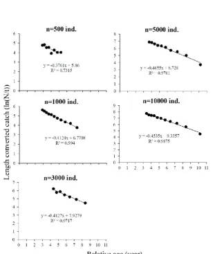
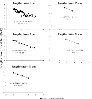
In this study, increasing sample size tended to raise the accuracy of the Z estimates except in the case of Z=0.40 year-1. In this case, a length interval size of 5 cm was taken as an example and the plots of relative age and length converted into catches among a series of sample sizes were drawn (Figure 2 and Table 3). For a sample size of 500 individuals, variation among the points of relative age–length-converted catch was large, while the range of relative ages used to estimate Z shortened. These factors may result in underestimating Z at small sample sizes.
By contrast, for sample sizes above 3000 individuals, the maximum relative age was about 10 years and the corresponding value of the catch-converted curve seemed to be lower. A relative age of 10 years in the simulations was overestimated, because a maximum age of eight years was assumed in this study. This result occurs because fish dynamics suffered from a lower Z of 0.40 year-1 and a greater proportion of older fish tended to be caught. An overestimated age with a lower value of the catch-converted curve would bias the estimation of Z. This explains why sample sizes above 3000 individuals in the cases of higher Z do not produce a biased Z value.
Table 2. The simulated mean Z, proportion error (E%), standard deviation (SD) and coefficient variation (CV) among 8 scenarios
initial Z Mean Z E% SD CV
S1
S1-1
0.40 0.42 4.78 0.02 0.04
0.60 0.60 -0.53 0.02 0.03
0.80 0.79 -1.38 0.04 0.05
1.00 0.97 -3.31 0.05 0.05
1.20 1.16 -2.99 0.06 0.05
S1-2
0.40 0.40 1.18 0.02 0.04
0.60 0.59 -2.36 0.02 0.03
0.80 0.81 1.04 0.04 0.04
1.00 1.00 0.02 0.05 0.05
1.20 1.19 -0.82 0.06 0.05
S1-3
0.40 0.45 11.76 0.02 0.04
0.60 0.62 2.64 0.02 0.04
0.80 0.84 4.67 0.04 0.04
1.00 0.98 -2.19 0.05 0.05
1.20 1.22 1.61 0.07 0.06
S1-4
0.40 0.40 0.03 0.02 0.04
0.60 0.56 -6.81 0.02 0.04
0.80 0.82 2.54 0.05 0.06
1.00 0.98 -2.16 0.05 0.05
1.20 1.49 24.20 0.11 0.07
S2
S2-1
0.40 0.38 -4.42 0.02 0.06
0.60 0.55 -7.77 0.02 0.04
0.80 0.74 -7.45 0.03 0.04
1.00 0.93 -6.93 0.04 0.04
1.20 1.13 -5.55 0.06 0.05
S2-2
0.40 0.36 -8.99 0.01 0.04
0.60 0.50 -16.52 0.02 0.04
0.80 0.69 -13.80 0.03 0.04
1.00 0.89 -11.42 0.04 0.04
1.20 1.08 -9.92 0.06 0.05
S2-3
0.40 0.32 -20.78 0.01 0.04
0.60 0.45 -25.70 0.02 0.04
0.80 0.63 -21.03 0.03 0.04
1.00 0.83 -17.09 0.04 0.05
1.20 1.02 -15.20 0.06 0.05
S2-4
0.40 0.27 -33.49 0.01 0.04
0.60 0.39 -34.71 0.02 0.04
0.80 0.58 -28.08 0.02 0.03
1.00 0.76 -23.89 0.03 0.04
1.20 0.96 -20.16 0.04 0.05
S3
S3-1
0.40 0.46 13.79 0.02 0.04
0.60 0.64 6.85 0.03 0.04
0.80 0.84 4.52 0.04 0.05
1.00 1.03 2.92 0.05 0.05
1.20 1.23 2.34 0.07 0.06
S3-2
0.40 0.50 25.09 0.02 0.04
0.60 0.69 15.22 0.03 0.04
0.80 0.89 10.76 0.04 0.05
1.00 1.08 8.12 0.06 0.05
1.20 1.28 6.53 0.08 0.06
S3-3
0.40 0.54 36.04 0.02 0.04
0.60 0.73 21.82 0.03 0.04
0.80 0.92 15.48 0.04 0.04
1.00 1.13 12.66 0.05 0.05
1.20 1.33 10.75 0.08 0.06
S3-4
0.40 0.58 45.19 0.02 0.03
0.60 0.77 27.82 0.03 0.04
0.80 0.96 20.40 0.05 0.05
1.00 1.16 15.73 0.06 0.05
et al., 2009). Such measurement error might bias the
Z estimates when a smaller length interval size is adopted. Smaller length interval sizes from 2 cm to 4 cm were considered in the simulations, but the results were similar to those provided when a length interval size of 5 cm was applied. A larger length interval size such as 5 cm might overcome the bias that results from measurement error. Therefore, without knowing the measurement error that influences the estimates of
Z when using the LCCM, a length interval size of 5 cm may be optimal for this method.
As recruitment levels decreased or increased, the
LCCM overestimated or underestimated Z
remarkably, and the results were the inverse for initial
Z changes over time. In the LCCM, the age composition of samples was a major determinant of the Z estimates. Recruitment history and total mortality can affect the age composition of the fish
Table 2. (Continued)
initial Z Mean Z E% SD CV
S4 S4-1 0.85 0.67 -20.89 0.03 0.05
S4-2 1.30 1.00 -23.27 0.06 0.06
S5 S5-1 0.40 0.71 78.55 0.03 0.04
S5-2 0.40 0.72 79.15 0.03 0.04
S6
S6-1 1.40 1.38 -1.21 0.07 0.05
S6-2 1.40 1.38 -1.29 0.08 0.06
S6-3 1.40 1.28 -8.81 0.09 0.07
S6-4 1.40 1.03 -26.35 0.07 0.07
S7 S7-1 0.65 0.63 -3.36 0.03 0.04
S7-2 0.65 0.60 -7.87 0.02 0.04
S7-3 0.65 0.56 -13.95 0.02 0.04
S7-4 0.65 0.51 -21.41 0.02 0.04
S8 S8-1 0.90 0.53 -41.26 0.02 0.04
S8-2 0.65 0.47 -28.12 0.02 0.04
population of the current year and thus Z may not be estimated accurately using the LCCM. In this study, fish populations suffered constant total mortality for
four successive years, which can remove the historical trend in total mortality. However, the bigeye tuna population in the Indian Ocean has suffered a sharply
Table 3. Comparison of the simulated Z values by sample size between the original age range and the modified age range using at estimating slope of Z=0.40 year-1 and length class=5 cm
Original age range and the simulated Z Modified age range and the simulated Z
Sample size Age range Z Age range Z
500 3.4~6.0 0.36 3.4~6.0 0.36
1000 2.6~7.5 0.39 2.6~6.9 0.40
3000 3.1~9.0 0.43 3.1~6.9 0.40
5000 3.1~10.2 0.45 3.1~6.9 0.40
10,000 3.2~10.2 0.47 3.2~6.9 0.40
Figure 3. The simulated plots of length converted catch values and relative ages among a series of sample sizes (Z=0.80 year-1 and length class=5 cm).
Table 4. Age range used to estimate Z for different levels of Z (sample size=3000 and length class=5 cm)
Sample size=3000; length class=5 cm
Z Age range Estimated Z E%
0.40 3.1~9.0 0.42 5.77
0.60 3.2~8.1 0.60 0.00
0.80 2.6~6.9 0.80 0.00
1.00 2.6~6.0 0.98 -1.95
decreasing trend in fishing mortality recently (0.43 year-1 in 2004 to 0.27 year-1 in 2008) (Nishida and Rademeyer, 2009). This situation is similar to S5-1 under the assumption of natural mortality=0.40 year-1, indicating using the LCCM would underestimate Z by 80% for the bigeye tuna population in the Indian Ocean if the effect of recruitment variation was not considered in the simulations, making the stock assessment too optimistic.
In conclusion, this study provided information on the non-equilibrium state of fish stocks that influences the estimation of Z when using the LCCM. We suggest that this method be adopted in situations when bigeye tuna populations undergo a stable fishing level for four successive years or when an approximate Z value of a fish stock is required. For bigeye tuna populations that are fully exploited and that are still undergoing high fishing pressure, the LCCM should be used to estimate the Z of this species with caution.
References
Castro, M., and Erzini, K. 1988. Comparison of two length-frequency based packages for estimating growth and mortality parameters using simulated samples with varying recruitment patterns. Fish. Bull., 86(4): 645-653.
Chen, S., and Watanabe, S. 1989. Age dependence of natural mortality coefficient in fish population dynamics. Bull. Jap. Soc. Sci. Fish., 55(2): 205-208. Chang, S.K., Lin, T.T., Lin, G.H., Chang, H.Y. and Hsieh,
C.L. 2009. How to collect verifiable length data on tuna from photographs: an approach for sample vessels. Ices J. Mar. Sci., 66(5): 907-915. doi: 10.1093/icesjms/fsp108
Erzini, K. 1990. Sample size and grouping of data for length frequency analysis. Fish. Res., 9(4): 355-366. Farley, J.H., Clear, N.P., Leroy, B., Davis, T.L.O. and
McPherson, G. 2006. Age, growth and preliminary estimates of maturity of bigeye tuna, Thunnus obesus, in the Australian region. Mari. Freshwater Res., 57(7): 713-724. doi: 10.1071/mf05255.
Hallier, J.P., Stéquert, B., Maury, O. and Bard, F.X. 2005. Growth of bigeye tuna (Thunnus obesus) in the eastern Atlantic Ocean from tagging-recapture data and otolith readings. Collect. Vol. Sci. Pap. ICCAT, 57(1): 181-194.
Hampton, J., and Majkowski, J. 1987. An examination of the reliability of the ELEFAN computer programs for length-based stock assessment, p. 203-216. In D. Pauly and G. R. Morgan (eds.) Length-based methods in fisheries Research. ICLARM Conf. Proc. 13, 468 pp.
Hoenig, J.M., Csirke, J., Sanders, M.J., Abella, A., Andreoli, M.G., Levi, D., Ragonese, S., Al-Shoushani, M. and El-Musa, M.M. 1987. Data Acquisition f or length-based stock assessment: report
of working group I, p.343-352. In D. Pauly and G. R. Morgan (eds.) Length-based method in fisheries research. ICLARM Conf. Proc. 13, 468pp.
Langley, A., Hampton, J., Kleiber, P. and Hoyle, S. 2008. Stock assessment of bigeye tuna in the western and central Pacific Ocean, including an analysis of management options. WCPFC-SC4-2008/SA-WP-1. http://www.wcpfc.int/doc/sa-wp-1/stock-assessment- bigeye-tuna-western-and-central-pacific-ocean-including-analysis-manage
Lehodey, P., Hampton, J. and Leroy, B. 1999. Preliminary results on age and growth of bigeye tuna (Thunnus Obesus) from the western and central Pacific Ocean as indicated by daily growth increments and tagging data. Working Paper BET-2, presented to the 12th Meeting of the Standing, New Cledonia, 18 pp. Nishida, T. and Rademeyer, R.A. 2009. Preliminary results
of SA of IO bet by ADMB-ASPM. IOTC-2009-WPTT-27.
http://www.iotc.org/files/proceedings/2009/wptt/IOT C-2009-WPTT-27.ppt
Nishida, T. and Shono, H. 2006. Updated stock assessment of bigeye tuna (Thunnus obesus) resource in the Indian Ocean by the age structured production model (ASPM) analyses (1960-2004). IOTC-WPTT-2006. http://www.iotc.org/files/proceedings/2006/wptt/IOT C-2006-WPTT-22.pdf
Okamoto, H., and Miyabe, N. 1999. Data collection and statistics of Japanese tuna fisheries in the Indian Ocean.IOTC-1999-WPDCS-10.
http://www.iotc.org/files/proceedings/1999/wpdcs/IO TC-1999-WPDCS
Pauly, D. 1980. On the interrelationships between natural mortality, growth-parameters, and mean environmental-temperature in 175 fish stocks. J. Conseil, 39(2): 175-192.
Pauly, D. 1983. Length-converted catch curve. A powerful tool for fisheries research
in the tropics (Part I). Fishbyte, 1: 9-13. Pauly, D., Moreau, J. and Abad, N. 1995. Comparison of
age-structured and length-converted catch curves of brown trout salmo trutta in 2 French rivers. Fish. Res., 22 (3-4): 197-204. doi: 10.1016/0165-7836(94)00323-o
Stéquert, B., and Conand, F. 2004. Age and growth of bigeye tuna (Thunus obesus) in the western Indian Ocean. Cybium, 28(2): 163-170.
Sparre, P. 1990. Can we use traditional length-based fish stock assessment when growth is seasonal? Fishbyte, 8(2): 29-32.
Zhu, G., Dai, X., Song, L. and Xu, L. 2011. Size at sexual maturity of bigeye tuna Thunnus obesus (Perciformes:scombridae) in the tropical waters: a comparative Analysis. Turk. J. Fish. Aquat. Sci., 11: 151-158.