Computation of a Minimum Average Distance Tree on
Circular-arc Graphs
Biswanath Jana
Department of Applied Mathematics with Oceanology and Computer Programming,
Vidyasagar University, Midnapore -721102, India.
Sukumar Mondal
Department of Mathematics, Raja N. L. Khan Women's College, Gope Palace, Paschim Medinipur -
721102, India.
Madhumangal Pal
Department of Applied Mathematics with Oceanology and Computer Programming,
Vidyasagar University, Midnapore -721102, India.
Abstract – The average distance of a finite graph 𝑮 = (𝑽, 𝑬) is the average of the distances over all unordered pairs of vertices. A minimum average distance spanning tree of G is a spanning tree of G with minimum average distance. Such a tree is sometimes referred to as a minimum routing cost spanning tree. In this paper, we present an efficient algorithm to compute a minimum average distance spanning tree on circular-arc graph in 𝑶(𝒏𝟐)time, where 𝒏 is the
number of vertices of the graph.
Keywords – Algorithms With Complexity, Circular-Arc Graphs, MAD Tree, Spanning Tree.
I.
I
NTRODUCTIONA graph G = (V, E) is called an intersection graph for a finite family F of a non-empty set if there is a one-to-one correspondence between F and V such that two sets in F
have non-empty intersection if and only if their corresponding vertices in V are adjacent to each other. We call F an intersection model of G. For an intersection model F, we use G(F) to denote the intersection graph for
G.
Intersection graphs have received much attention in the study of algorithmic graph theory and their applications [1]. Well-known special classes of intersection graphs include interval graphs, chordal graphs, circular-arc graphs, permutation graphs, circle graphs and so on. If F is a family of arcs on a circle, then G is called a circular-arc graph for F and F is called a circular-arc model of G. If F
is a family of line segments on real line, then G is called an interval graph for F.
Let S = {C1, C2, ...,Cn}be a family of n arcs on a circle
C. Each endpoint of the arcs in assigned to a positive integer, called a coordinate. The endpoints of each arc are located on the circumference of C in the ascending order of the values of the coordinates in the clockwise direction. For convenience, each arc Ci, i = 1, 2, ..., n, is
represented as (hi,ti), where hi (the head) and ti (the tail)
denote, respectively that starting and ending points of the arc when it is traversed in counter clockwise manner, starting with an arbitrary chosen point on C which is not an endpoint of any arc in S. Without loss of generality, we assume the following:
(i) no single arc in S covers the entire circle C by itself, (ii) no two arcs share a common endpoint,
(iii) 𝑛𝑖=1𝐶𝑖 = 𝐶 (otherwise, the problem becomes one on
interval graph),
(iv)the arcs are sorted in increasing values of ti's, i.e.,ti>tj
for i>j.
Also the family of arcs S is said to be canonical ifhi's
and ti's for i = {1, 2, ..., n} are all distinct integers.
A path of a graph G is an alternating sequence of distinct vertices and edges, beginning and ending with vertices. The length of a path is the number of edges in the path. A path from vertex i to j is a shortest path from i to j
with lower length. The shortest distance (i.e., the length of the shortest path) between the vertices i and j is denoted by 𝑑𝐺(𝑖, 𝑗).
Alternatively, a circular-arc graph can be defined as follows:
An undirected graph G = (V, E) is a circular-arc graph if and only if
(i) its vertices circularly indexed as v1, v2, ...,vn and
(ii)(vi,vj) E, provided Ci and Cjintersect with each other,
where vi and vj are the vertices in the graph G
corresponding to the arcs Ciand Cj respectively.
It may be noted that the arc Ci and the vertex vi or i are
one and the same thing.
Circular-arc graphs have applications in genetic research [2], traffic control [3], etc. This class of graphs admits some interesting subclasses:
(1) Proper circular-arc graphs: a graph G is a proper circular-arc (PCA) graph if there is a circular-arc representation of G such that no arc is properly contained in any other.
(2) Unit circular-arc graphs: a graph G is a unit circular-arc (UCA) graph if there is a circular-circular-arc representation of
G such that all arcs are of the same length.
Clearly, it can be easily proved that UCA PCA. In [4], the author showed that this inclusion is strict. An example of a PCA graph which is not a UCA graph has also been given by Golumbic [1].
(3) Helly circular-arc graphs: A family of subsets S satisfies the Helly property when every subfamily of it consisting of pairwise intersecting subsets has a common element. So, a graph G is a Helly circular-arc (HCA) graph if there is a circular-arc representation of G such that the arcs satisfy the Helly property.
(4) Clique-Helly circular-arc graphs: a graph G is a clique-Helly arc (CH-CA) graph if G is a circular-arc graph and a Helly graph. A graph is clique-Helly when its cliques satisfy the clique-Helly property.
Copyright © 2015 IJECCE, All right reserved Fig.1. A circular-arc graph G.
Fig.2. Circular-arc diagram of the circular-arc graph G of Figure 1.
Breadth-first-search (BFS) is a strategy for searching in a graph when search is limited to essential two operations: (a) visit and inspect a node of a graph; (b) gain access to visit the nodes that neighbour the currently visited node. The BFS begins at a root node and inspect all the neighbouring nodes. Then for each of those neighbour nodes in turn, it inspects their neighbour nodes which were unvisited, and so on.
BFS is a uniformed search method that aims to expand and examine all nodes of a graph or combination of sequences by systematically searching through every solution. In other words, it exhaustively searches the entire graph or sequence without considering the goal until it finds it.
Let G be a connected undirected graph, let v be a vertex of G and let 𝑇 be its spanning tree obtained by the BFS of
G with the initial vertex v. An appropriate rooted tree
𝑇 𝑣 = 𝑉, 𝐸′ ⊆ 𝐺 let us call a Breadth-First-Search
Tree (BFS tree, for short) with the root v, the edges of G that do not appear in BFS tree let us call non-tree edges.
In an un-weighted tree T = (V,E), the eccentricity e(v) of the vertex v is defined as the distance fromv to a vertex farthest from v inT, i.e.,e(v) = max {d(v, vi), vi T },
whered(v, vi) is the number of the edges on the shortest
path between v and vi.
In a weighted tree T = (V, E ), the eccentricity e(v) of the vertex v is denoted as sum of the weights of the edges fromv to a vertex farthest from v T , i.e.,e(v) = max {d(v, vi), vi T },
Where d(v, vi) is the sum of the weights of the edges on
the shortest path between v and vi.
A vertex with minimum eccentricity in the tree T is called a center of that tree T, i.e., if e(s) = min{e(v), for all
vV}, then s is the 1-center. It is fact that every tree has
either one or two centers vertices which is classical result for unweighted trees. However, if weighted trees are considered, then this is only true if all edge-weights are strictly positive. Recently, Jana et al. [7] have designed an efficient algorithm to compute inverse 1-center location on the weighted trees which takes O(n) time.
The eccentricity of a center in a tree is defined as the radius of the tree and is denoted by (T ), i.e.,
𝜌 𝑇 = {minv∈T𝑒 𝑣 }
The diameter of a tree T is denoted as the length of the longest path in T, i.e., the maximum eccentricity is the diameter. A spanning tree with minimum diameter is defined as minimum diameter spanning tree.
The average distance (G) of a circular-arc graph G = (V, E) is the average over all unordered pairs of vertices of the distances,
𝜇 𝐺 = 2
𝑛(𝑛 − 1) 𝑑𝐺
𝑢,𝑣∈𝑉(𝐺)
(𝑢, 𝑣)
where𝑑𝐺(𝑢, 𝑣)denotes the distance betweenthe vertices u
and v, i.e., the length of a shortest path joining the vertices
u and v.
The minimum average distance spanning tree (MAD tree, for short) of a circular-arc graph G is a spanning tree of G with minimum average distance.
1.1 Survey of the Related Work
In general, the problem of finding a MAD tree is NP-hard [8]. A polynomial time approximation scheme is due to [9]. Hence it is natural to ask for which restricted graph classes a MAD tree can be found in polynomial time. In [10], an algorithm is exhibited that computes a MAD tree of a given distance-hereditary graph in linear time. Recently, Dahlhaus et al. [11], have design a linear time algorithm to compute a MAD tree of an interval graph which runs in O(n) time when the left and right boundaries of the intervals are ordered. In [12], Barefoot et al., have shown that if T is a MAD tree of a given connected graph
G, then there exists a vertex c in T such that every path in
T starting at c is induced in G. It remains an open problem to decide whether there exists a polynomial time algorithm to neighbourhood a MAD tree of a vertex weighted interval graph. Olario et al. [13], have design optimal parallel algorithms for problems modelled by a family of intervals on interval graphs to compute a MAD tree. Recently, Jana et al. [14], and Mondal [15] have designed an efficient algorithms to compute minimum average distance spanning tree on permutation graphs and trapezoid graphs respectively in O(n2) time, where n is the number of vertices of the graph.
1.2 Applications of the problem
MAD trees, also referred to as minimum routing cost spanning trees, are of interest in the design of communication networks [8]. One is interested in designing a tree subnetwork of a given network, such that on average, one can reach every node from every other node as fast as possible.
1.3 Our result
1.4 Organization of the paper
In the next section, i.e., Section 2, we present the construction of the tree. In Subsection 2.1, we present BFS tree on circular-arc graph and in Subsection 2.2, we present the minimum diameter spanning tree. In Subsection 2.3, we develop modified spanning tree of the tree T. In Section 3, we discuss about average distance. In subsection 3.1, we present the algorithm to compute average distance. In Section 4, we present an algorithm to get MAD tree of the circular-arc graph. The time complexity is also calculated in this section and Section 6 presents conclusion of the work.
II.
C
ONSTRUCTION OF THET
REE2.1 Construction of BFS tree on circular-arc graph
It is well known that BFS is an important graph traversal technique and also BFS constructs a BFS tree. In BFS, started with vertex v, we first scan all edges incident on v
and then move to an adjacent vertex w. At w we then scan all edges incident to w and move to a vertex which is adjacent of w. This process is continued till all the edges in the graph are scanned.
BFS tree can be constructed on general graphs in
O(n+m) time, where n and m represent respectively the number of vertices and number of edges [3]. To construct this BFS tree on a circular-arc graph we consider the circular-arc diagram. We first number the vertices of the circular-arc graph successively by 1, 2, 3, ..., n
corresponding to the circular arcs C1, C2, ...,Cn
according to the order of end pointsti (the tail) of the
circular arcsrespectively when it is traversed in clockwise manner. To construct the rooted tree, we traverse the graph in anticlockwise manner. Firstly, we placed the vertex corresponding to the maximum length of the arcs Ci (i ≠1),
which are adjacent to the arc C1, as a root and put in zero level. Then we traverse all vertices (corresponding to arcs) adjacent to Ciand placed them on the first level. Next we
traverse the circular-arc diagram step by step until all vertices corresponding to the arcs are traversed. In this way, we get a left BFS tree, denoted by TL(i). Secondly,
we construct BFStree by same manner traversed in clockwise direction of the vertex corresponding to the arc C1placed the maximum length of the arcs Cj(j ≠ 1), which
are adjacent to the arc C1, as a root and put in zero level and all vertices (corresponding to arcs) adjacent to Cjon
the first level. Next we traversed the circular-arc diagram step by step. In this way, we get a right BFS tree, denoted by TR(j). Figure 3(a) and 3(b) represent the left BFS trees
TL(7) rooted at the vertex 7 corresponding to the arc C7and
a right BFS tree TR(2) rooted at the vertex 2 corresponding
to the arc C2, respectively of the circular-arc graph shown
in Figure 1. By the following algorithm one can design the BFS tree on circular-arc graphs.
Now, we define level of the vertex v as the distance of v
from the root i of the BFS tree T(i) and denote it by
level(v), v V and take the level of the root i as 0. The level of each vertex of the tree Tcan be computed in O(n) time.
(a) (b)
Fig.3. BFS trees TL(7) and TR(2) rooted at vertices 7 and 2 respectively of the circular-arc graph shown in Figure 1.
Algorithm CARBFS-TREE
Input:
Sorted arcs Ci, i = 1, 2, …., n with endpoints (hi,ti)of the circular-arc diagram of thecircular-arc graph G = (V, E).
Output:
BFS tree with root j, TR(j).Step 1:
Compute the adjacent arcs to the arc C1and selectthe arc of maximum tails tj of thoseadjacent arcs in
clockwise sense.
Step 2:
Choose the vertex j corresponding to the arc Cjasroot of the tree. Then find the adjacentvertices to j and placed them as leaves at level 1, and mark them.
Step 3:
Let k be the vertex corresponding to the arc Ck with maximum tail tk among the tails ofadjacent arcs to Cj. Then put k as node on main path.
Next find all other unmarked adjacent arcs to Ckand they
are placed as leaves at level(k)+1. Mark them.
Step 4:
This process continued until all arcs are marked. end CARBFS-TREE.By similar way we can construct the BFS tree with root i
in anticlockwise manner, i.e. TL(i). The time complexity of
the Algorithm CARBFS-TREE is stated below.
Theorem 1:
The BFS trees TR(j) and TL(i) rooted at anyvertex x V can be computed in O(n) timefor a circular-arc graph containing n vertices.
Proof.
Step 1 of the above algorithm can be computed in O(n) time, because sorted arcs and adjacent arcs are finite. In Step 2, selection of the root j takes O(1) time and to mark the vertices adjacent to jtakes O(n) time. Therefore, Step 2 runs in O(n) time. Also computation of the vertex kcorresponding to the maximum tail among the tails of the arcs adjacent to the arc Cjtakes O(n) time. So, Step 3 takes O(n) time. Since Step 4 is the checking step, so it takes O(n) time. Hence, over all the time complexity of Algorithm CARBFS-TREE is O(n) time, where n is the number of vertices. □Obviously, two BFS trees, each contains n vertices and
(𝑛 − 1) edges corresponding to the given circular-arc
graph with n vertices. So, it is a spanning tree.
2.2 Computation of minimum diameter spanning tree
Let TL(i) and TR(j) be two BFS trees of a circular-arc graphG. Next we determine the diameters of the trees TL(i) and
TR(j). If the diameter of TL(i) is less than the diameter of
TR(j), then we denote TL(i)
Copyright © 2015 IJECCE, All right reserved diameter between the trees TL(i) and TR(j).
Let P be the path in the BFS tree T with maximum length of the circular-arc graph G, defined as main path and it is denoted by u1*→u2* → u3* → …… → uK*
corresponding to the arcs C1*, C2*, C3*, ……., CK*, where k
≤ n. Also, ui *
, i = 1, 2, 3, …, k are nodes in the main path
P. Now, we define some more terms below.
The open neighbourhood of the vertex 𝑢𝑖∗in the path P
of G, denoted by 𝑁 𝑢𝑖∗ and defined as
𝑁 𝑢𝑖∗ = {𝑢′′: 𝑢′′, 𝑢𝑖∗ ∈ 𝐸}
and the closed neighbourhood
𝑁[𝑢𝑖∗] = 𝑁 𝑢𝑖∗ ∪ {𝑢𝑖∗},
whereEis the edge set of the given circular-arc graph. As per construction of BFS tree we have the following important results in BFS tree T.
Lemma 1:
If u, v V and |level(u) - level(v)| > 1 in T, then there is no edge between the vertices u and v in G, except such (u, v) E in which level(u) = 1 and level(v) = k, where k is the highest level.Proof.
If possible, let |level(u) - level(v)| > 1 but (u, v) E, i.e., u and vare directly connected. Since u and v are directly connected so by the idea of breath first search, at any stage if u and v are theadjacent to the previously visited vertex, then u and v to be placed in same level, so
level(u) = level(v).But, if u is adjacent to a previously visited vertex then v must be adjacent to next visited vertex,and then v to be placed in the next level in T. So, in this case |level(u) - level(v)| = 1. Thus, eitherlevel(u) = level(v) or |level(u) - level(v)| = 1 implies (u, v) E, which is contradictory to the assumption |level(u) - level(v)|> 1, (u, v) E.
By the process of the ordering of the arcs of the circular-arc graphs it is evident that there is at least one circular-arc which is extended on both sides of the fixed line (dotted line in Figure 2) from which order of the arcs begins. So one end vertex of the edge (u, v) E of Gis at either in first level, i.e., at level 1 or in highest level, i.e., at level k.Hence the result.□
Now, we shall prove that the BFS tree is a minimum diameter spanning tree.
Lemma 2.
The spanning tree T is a minimum diameter spanning tree.Proof.
According to the construction the BFS tree, the main path of the tree T is the longest path which is the diameter of T. The main path covers thewhole circle with least number of arcs. This diameter is minimum, because Tis the minimum height tree. Also, T is a spanning tree. Hence Tis a minimum diameter spanning tree. □
In next subsection, we shall discuss about the modified spanning tree T′of the spanning tree T.
(a) (b)
Fig.4. Isomorphic trees T1L(7) and T1R(2) of the BFS trees TL(7) and TR(2) respectively, where main path is
horizontal.
2.3 Modification of the spanning tree T
It is observed that T is not necessarily a MAD tree. So, modification of T is necessary. We modify T by the following way:
First, we draw the tree T1 (shown in Figure 4(a) and
Figure 4(b)) whose main path is horizontal and isomorphic to the tree T. Then, we compute N(ui*) G for each
vertices on the main path P. If there are any common adjacent vertices of two nodes ui*and ui+1* in the main path
P, where 𝑖 = 1, 2, . . . , 𝑘 − 1 then we can shift them by the following way.
Step I:
In G, if any common adjacent vertex w ofui*and ui+1*exist, then we calculate the number of vertices
k1, k2 respectively, onthe both sides separately of the node
ui*(taken as fixed and leaves which does not lie on main
path are not countable) in T1along the main path.
Next, calculate their difference, say,
d1= |k1- k2|.
Step II:
Again, find the number of vertices on the both sides separately of the node ui+1*(taken as fixed) inT1along the main path(ignoring the vertex obtained in Step
I).
Next, calculate their difference, say, d2.
Step III:
Case-I: If d1- d2< 0, then unaltered, i.e. wremains adjacent of ui*in T1.
Case-II: If d1 = d2, then calculate
D1= 𝑢,𝑣∈𝑉(𝑇1)𝑑𝑇1(𝑢, 𝑣)
(total distance before shifting) and
D2 = 𝑢,𝑣∈𝑉(𝑇1)𝑑𝑇1(𝑢, 𝑣) (total distance after shifting).
If D1<D2then, tree remains unaltered else w is shifted.
Case-III: If d1- d2> 0, then the adjacent vertex w of the
node ui *
is shifted to the nodeui+1 *
,i.e.,wis finally adjacent to ui+1*in T1.
Step IV:
Finally represent T1as form of tree T′ .
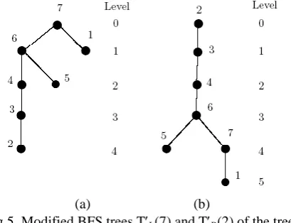
Similar idea is used for pair of any two nodes on the main path P. Using this method we construct the modified spanning tree T′ starting from T with the help of T1. Figure
5(a) and Figure 5(b) are the modified BFS trees T′L(7) and
T′R(2) of the BFS trees TL(7) and TR(2) respectively
(shown in Figure 3(a) and Figure 3(b) respectively).
Lemma 3:
If T′is a BFS tree, then the distance𝑑𝑇′ 𝑢, 𝑣 between the vertices u and v in T′ is given by
𝑑𝑇′ 𝑢, 𝑣
=
𝑙𝑒𝑣𝑒𝑙 𝑣 , if 𝑢 is a root and 𝑣 is any vertex,
𝑙𝑒𝑣𝑒𝑙 𝑢 − 𝑙𝑒𝑣𝑒𝑙 𝑣 , if 𝑢and v both are
nodes in main path P, 𝑙𝑒𝑣𝑒𝑙 𝑝𝑎𝑟𝑒𝑛𝑡 𝑢 − 𝑙𝑒𝑣𝑒𝑙 𝑣 + 1, if 𝑢 is any
leaf and 𝑣 is any node in P.
Proof. Case I:
If uis a root.In the tree T′, with u as root there exists a unique shortest path u → z1→ z2→….. → zp-1 →vfrom u to any vertex v G, where u is the parent of z1 and zi is the parent
of zi+1 and so on for each i = 1, 2, ……, p - 2 and zp-1 is the
Next we are to show that 𝑑𝑇′ 𝑢, 𝑣 ≮ 𝑝. If possible, let
dT′ (u, v)= q < p. Then there exist apath u → y1→ y2→….. → yp-1 →vfrom u to any vertex v G. As each vertex of this path is directly connected with the next one, level(y1) is either 0 or 1 since level(u) = 0 and level(yk+1) is either level(yk) or level(yk) + 1 or level(yk) - 1. Thus level(y2) is 0 or 1 or 2, level(y3) is 0 or 1 or 2 or 3 and so on.
Therefore level(v) is 0 or 1 or 2 or...or q. This is a contradiction since level(v) = p and p > q. Hence
𝑑𝑇′ 𝑢, 𝑣 ≮ 𝑝, which implies 𝑑𝑇′ 𝑢, 𝑣 = 𝑝, i.e. dT′ (u, v)=
level(v).
(a) (b)
Fig.5. Modified BFS trees TL(7) and TR(2) of the trees TL(7) and TR(2) respectively shown in Fig. 3.
Case II:
If u and vboth are nodes in the main path P.If u and v both are the nodes in the main path P, then as per rule of construction of BFS, there is a shortest pathu
→ z1′→ z2′→….. → zp-1′ →v. Here z1′ is at next level of u, z2
′
is at the next level of z1 ′
and so on uptov. Let level of u
be i, so d(u, z1′) = 1 = (i + 1) - i = level(z1′) - level(u), d(u, z2′) = d(u, z1′) + d(z1′, z2′) = 1 + 1 = 2 = (i + 2) - i = level(z2′) - level(u). If d(u, zk′) = k = (i + k) - i = level(zk′) - level(u), then d(u, zk+1′) = d(u, zk′) + d(zk′, zk+1′) = k + 1 = (i + k + 1) - i = level(zk+1′) - level(u). Hence
dT′ (u, v) = |level(v) - level(u)|.
Case III:
If u is any leaf and v is any node in the main path P.In this case, there is a path from u to v via the parent of u. If level(u) = i, then level(parent(u)) = i -1and parent(u) is a node in the main path P (as per construction of BFS rooted at the vertex corresponding to the arc x with maximum length of the arc 1 in anticlockwise manner or the vertex corresponding to the arc y with maximum length of the arc 1 in clockwise manner). Therefore dT′ (u,v)= d(u, parent(u)) +d(parent(u), v) = 1 + level(v) - level(parent(u)), i.e.,dT′(u, v)= |level(parent(u)) - level(v)|
+ 1.□
III.
A
VERAGED
ISTANCEMany works on average distance in graphs are available in literature [16, 17, 18, 19, 20, 21]. Chung [22] give a bound of average distance of a graph in terms of independent number. She has shown that (G) (G), where (G) and (G) denote respectively the average distance and the independent number of the graph G. Also in [23], the average distance of an interval graph with
edges of unit length can be computed inO(m) time where m is the number of edges. In this section, we discuss about the computation of average distance of a circular-arc graph.
The average distance (G) of a connected circular-arc graph G = (V, E) is the average over all unordered pairs of vertices of the distances,
𝜇 𝐺 = 2
𝑛(𝑛 − 1) 𝑑𝐺
𝑢 ,𝑣∈𝑉(𝐺)
(𝑢, 𝑣)
where𝑑𝐺(𝑢, 𝑣) denotes the distance between the vertices u
and v, i.e., the length of a shortest path joining the vertices
u and v. The average distance can be used as a tool in analytic networks where the performance time is proportional to the distance between any two nodes. It is a measure of the time needed in the average case, as opposed to the diameter, which indicates the maximum performance time.
3.1 Algorithm to compute average distance and its
computation
At first we compute dG(u, v) for every pair u, v (u ≠ v),
then we compute the sum of distance between all pairs of vertices and finally we multiply it by the factor 2
𝑛(𝑛−1)
to get the average distance. From above procedure it follows that the time to compute the average distance is same as the time to compute all pairs shortest distances. The average distance of a circular-arc graph can be computed in sequential using O(n2) time, where n is the number of vertices of the graphs.
IV.
A
LGORITHM AND ITSC
OMPLEXITY In this section, we present an efficient algorithm to construct MAD tree for a given circular-arc graph. Also, the correctness of the algorithm and its time complexity are presented here.Algorithm CAMAD-TREE
Input:
Sorted endpoints of the arcs S = {C1,C2, ....,Cn}of the circular-arc graph G = (V, E).
Output:
MAD tree Tand average distance (T‟).Step 1:
Compute the minimum diameterspanning treeT//by Section 3.2//and
Calculate level(u) = d(u’, u),u’is either the vertex corresponding to the left maximum spread arc of the arc
C1 or the vertex corresponding to the right maximum
spread arc of the arc C1.
Step 2:
Compute N(ui) for all ui T andk = height of the tree T
= highest level.
Step 3:
//Modification of the tree T //Compute common vertices, if any, of two internal nodes ui
and ui+1; i = 0, 1,2, ...., k – 1of the main path P may be
shifted as leaves to the node ui+1
under following conditions otherwise remains unaltered.
Step 3.1:
For i = 0 to k - 1 doifN(ui) N(ui+1) = then go to Step 3.1,
ifN(ui ) N(ui+1)≠ and let
Copyright © 2015 IJECCE, All right reserved
Step 3.1.1:
Calculate the numberof verticesto one sideand other side of the internal node ui in T with ui as origin.
Next calculate theirdifference, d1.
Step 3.1.2:
Calculate the numberof vertices to one sideand other side of theinternal node ui+1 in T with ui+1asorigin (ignoring the vertex w). Next calculate their difference, d2.
Step 3.1.3:
If d1 - d2< 0, thenunaltered;ifd1 - d2 = 0,then calculate
D1 = 𝑑𝑇(𝑢, 𝑣) (totaldistance before shifting) and
D2= 𝑑𝑇 𝑢, 𝑣 (total distance aftershifting) and
consider minimum{D1, D2 },
ifd1- d2> 0, then the adjacent vertex w of the internal node
ui is shifted to the internal node ui+1.
Step 3.2:
Set T as modified spanning tree of T on circular-arc graph G.Step 4:
Calculate 𝑑𝑇′ 𝑢, 𝑣=
𝑙𝑒𝑣𝑒𝑙 𝑣 , if 𝑢 is a root and 𝑣 is any vertex, 𝑙𝑒𝑣𝑒𝑙 𝑢 − 𝑙𝑒𝑣𝑒𝑙 𝑣 , if 𝑢and v both are nodes in
main path P, 𝑙𝑒𝑣𝑒𝑙 𝑝𝑎𝑟𝑒𝑛𝑡 𝑢 − 𝑙𝑒𝑣𝑒𝑙 𝑣 + 1, if 𝑢 is any leaf and
𝑣 is any node in P.
and 𝜇 𝑇′ = 2
𝑛(𝑛−1) 𝑢,𝑣∈𝑉(𝑇′)𝑑𝑇′(𝑢, 𝑣) end CAMAD-TREE
4.1 Illustration of the algorithm
In Figure 4(a), ui* = 7 andui+1* = 6 are two nodes. 5 is
the common adjacent of the vertices ui *
and ui+1 *
, i.e., w = 5. Taking the vertex 7 as fixed, the number of vertices on the both sides of the node 7 in T1L(7) along the main path
are 4 and 1. Hence their difference is d1 = 4 - 1 = 3. Again
takingthe vertex 6 as fixed, the number of vertices on the both sides of the node 6 in T1L(7) along the mainpath is 3
and is 2(ignoring the vertex 5) when the vertex 5 is adjacent with the vertex 6. Hence theirdifference is d2 = 3
- 2 = 1. Therefore d1> d2. So, the vertex 5 is shifted to the
node 6. Then we havethe modified spanning tree
T′L(7)(Figure 5(a)).
Next calculate the average distance μ1(G) corresponding
to the tree TL(7)(isomorphic to T1L(7)). Again calculate
average distance μ′1(G) corresponding to the tree T ′
L(7).
Here μ1(G) = 52/21 and μ′1(G) = 50/21. Clearly, μ1(G)
>μ′1(G). Hence T′L(7) is a minimum average distance tree
of the circular-arc graph G.
In Figure 4(b), which is the spanning tree TR(2) of the
circular-arc graph G with vertex 2 corresponding to the arc
C2 with maximum length adjacent to the arc C1 as root. ui*
= 2 and ui+1* = 7 are two nodes. 1 is the common adjacent
of the vertices ui*and ui+1*, i.e., w = 1. Taking the vertex 2
as fixed, the number of vertices on the both sides of the node 2 in T1R(2) along the main path are 0 and 5. Hence
their difference is d1 = 5 - 0 = 5. Again taking the vertex 7
as fixed, the number of vertices on the both sides of the node 7 in T1R(2) along the main path are 5 (ignoring the
vertex 1) and 0 when the vertex 1 is adjacent with the vertex 7. Hence their difference is d2 = 5 - 0 = 5.
Therefore d1 = d2, i.e., d1- d2 = 0. Then calculate D1 = 52
(total distance before shifting) and D2 = 50 (total distance
after shifting) and then consider minimum{D1,D2} = D2.
So, the vertex 1 is shifted to the node 7. Then we have the modified spanning tree T′R(2) (Figure 5(b)).
Next calculate the average distance μ2(G) corresponding
to the tree TR(2)(isomorphic to T1R(2)). Again calculate
average distance μ′2(G) corresponding to the tree T′R(2).
Here μ2(G) = 52/21 and μ′2(G) = 50/21.
Clearly, μ2(G)> μ′2(G). Hence T′R(2) is the another
minimum average distance tree of the circular-arc graph
G.
Next we shall show that for any circular-arc graph, the tree designed by the Algorithm CAMAD- TREE represents a MAD tree.
Theorem 2:
For any circular-arc graph, the tree designed by the Algorithm CAMAD-TREE is a MAD tree.Proof.
Let G = (V, E) be any circular-arc graph. Then, using Section 2.2, one can design a minimum diameter spanning tree. In this minimum diameter spanning tree, shifting (if necessary, under conditions stated in Section 2.3) of the some vertices to its next adjacent node in the main path means that those vertices are placed on such side of the tree, with respect to the fixed node in the main path, in which that side contains maximum number of vertices. As a result, after all possible shifting of the vertices,the sum of total distances over all unordered pair of vertices decreases. Thus the average distance of the tree decreases. Hence, the tree designed by the Algorithm CAMAD-TREEis a MAD tree for any circular-arc graph. This completes the proof. □Lastly, we describe the time complexity of the algorithm.
Theorem 3:
The MAD tree of a circular-arc graph Gwith n vertices can be computed in O(n2) time.
Proof.
Step 1 of Algorithm CAMAD-TREE takesO(n) time (Theorem 1). Step 2, i.e. computationof open neighbourhood of all nodes on the main path can be computed in O(n2) time. Each Step 3.1.1 and Step 3.1.2 takes O(n) time. Also Step 3.1.3 runs in O(n) time. But Step 3.1 repeats (k -1) times, so the total time complexity of Step 3.1 is O(n2), where k is of O(n). Again Step 3.2, i.e. modification of the tree can be computed in O(n2)time. The last step, i.e. Step 4, in worst case, can be computed in
O(n2) time. Hence, overall time complexity of our proposed algorithm is O(n2) time.
V.
C
ONCLUSIONIn this paper, we proposed an efficient algorithm to compute a minimum average distance spanning tree
on circular-arc graphs which is designed based on BFS technique. The time complexity of this algorithm is of 𝑂(𝑛2), where n is the number of vertices of the
A
CKNOWLEDGMENTSWe are very grateful to two anonymous referees for their many helpful and valuable comments to improve this paper. This work is in part supported by the UGC under the Major Research Project: F. No.41-764/2012 (SR) for second author.
R
EFERENCES[1] Golumbic, M. C., Algorithmic graph theory and perfect graphs, Academic Press, New York, 2000.
[2] Stahl F., Circular genetic maps, J. Cell Physiol, 70 (Suppl. 1) (1967) 1 – 12.
[3] Tarjan, R. E., Depth rst search and linear graph algorithm, SIAM J. Comput., 2 (1972) 146 - 160.
[4] Tucker, A., Structure theorems for some circular-arc graphs, Discrete Mathematics, 7 (1974) 167 - 195.
[5] Tucker, A., An efficient test for circular-arc graphs, SIAM J. Comput., 9 (1980) 1 - 24.
[6] Deng, X., Hell, P. and Huang, J., Linear time representation algorithms for proper circular-arc graphs and proper interval graphs, SIAM J. Comput., 25 (1996) 390 - 403.
[7] Jana, B., Mondal, S. and Pal, M., Computation of inverse 1-center location problem on the weighted trees, CiiT International Journal of Networking and Communication Engineering, 4 (2012) 70 - 75.
[8] Johnson, D. S.,Lenstra, J. K. and Rinnooy-Kan, A. H. G., The complexity of the network design problem, Networks, 8 (1978) 279 – 285.
[9] Bang Ye We, Lancia, G., Bafna, V., Chao, K. M., Ravi, R. and Chuang Yi Tang, A polynomial time approximation scheme for minimum routing cost spanning trees, SIAM Journal on Computing, 29 (1999) 761 - 778.
[10] Dahlhaus, E., Dankelmann, P., Goddard, W. and Swart, H. C., MAD trees and distance-hereditary graphs, Discrete Applied Mathematics, 131 (2003) 151 - 167.
[11] Dahlhaus, E., Dankelmann, P. and Ravi, R., A linear time algorithm to compute a MAD tree of an interval graph, Information Processing Letters, 89 (2004) 255 - 259.
[12] Barefoot, C. A., Entringer, R. C. and Szekely, L. A., Extremal values of distances in trees, Discrete Applied Mathematics, 80 (1997) 37 - 56.
[13] Olariu, S., Schwing, J. and Zhang, J., Optimal parallel algorithms for problems modeled by a family of intervals, IEEE Transactions on parallel and Distributed Systems, 3 (1992) 364 - 374.
[14] Jana, B. and Mondal, S., Computation of a Minimum Average Distance Tree on Permutation Graphs, Annals of Pure and Applied Mathematics, 2 (No. 1) (2012) 74 - 85.
[15] Mondal, S., An efficient algorithm for computation of a minimum average distance tree on trapezoid graphs, Journal of Scientific Research and Reports, 2 (2013) 598 - 611.
[16] Althofer, I., Average distance in undirected graphs and the removal of vertices, J. Combin. Theory Ser. B, 48 (1990) 140-142.
[17] Bienstock, D. and Gyon, E., Average distance in graphs with removed elements, J. Graph Theory, 12 (1988) 375 - 390. [18] Favaron, O., Kouider, M. and Maheo, M., Edge-vulnerability
and mean distance, Networks, 19 (1989) 493 - 504.
[19] Hendry, G. R. T., On mean distance in certain classes of graphs, Networks, 19 (1989) 451 - 557.
[20] Mohar, B., Eigenvalues, diameter and mean distance in graphs, Graphs and Combinatories, 7 (1991) 53 - 64.
[21] Winkler, P., Mean distance in a tree, Discrete Applied Math., 27 (1990) 179 – 185.
[22] Chung, F. R. K., The average distance and independence number, J. Graph Theory, 12 (1988) 229- 135.
[23] Dankelmann, P., Computing the average distance of an interval graphs, Information Processing Letters, 48 (1993) 311 - 314.
A
UTHOR'
SP
ROFILEBiswanath Jana
was born in Paschim Medinipur, West Bengal, India on 8th day of January, 1980. He received his Bachelor of Science degree with Honours in Mathematics from Vidyasagar University, West Bengal, India in 2002and he has passed Master of Science (Applied Mathematics) in Mathematics with first class from same University in 2004. He received his Bachelor of Education degree in 2006 from same University.
Currently he is an Assistant Teacher in Mathematics of Jhargram Bikash Bharati Sikshayatan, Jhargram, Paschim Medinipur, West Bengal, India.
Email: [email protected]
Sukumar Mondal
was born in Paschim Medinipur, West Bengal, India on the fifth day of September, 1971. He received his Bachelor of Science degree With Honours in Mathematics(rank second) from Vidyasagar University, West Bengal, India in 1992 and he stood first class second in Master of Science (Applied Mathematics) degree in 1994 from same University. He received his Bachelor of Education degree in 1996 from same University. He joined the department of Applied Mathematics with Oceanology and Computer Programming, Vidyasagar University, Midnapore, West Bengal, India, as a Junior Research Fellow on August 1997 and started research work for his Ph. D. degree. He was also awarded an individual research fellowship by Council of Scientific and Industrial Research, Govt. of India in 1997. He is currently A Ph. D. candidate in the department of Applied Mathematics with Oceanology and Computer Programming, Vidyasagar University, West Bengal, India. He was a Reader of department of Mathematics of Yogada Satsangha Palpara Mahavidyalaya, Palpara, Purba Medinipur, West Bengal, India. He has guided one research scholars for Ph.D. degrees and has published more than 20 articles in international journals and the member of the editorial Boards of the journal „Annals of Pure and Applied Mathematics‟. His specializations include Computational Graph Theory. He is also a reviewer of several international journals. He is the author of the books “Advanced Analytical Statics” published by U. N. Dhaur and Sons, Kolkata and “Advanced Hydrostatics” published by “Amit Publication”, Kolkata. Currently he is Associate Professor of Dept. of Mathematics of Raja N. L. Khan Women‟s College, Medinipur, West Bengal.
Email: [email protected] , India.