Evolving functional and structural dynamism in coupled boolean networks

Evolving Functional and

Structural Dynamism in

Coupled Boolean Networks

Larry Bull*

University of the West of England

Keywords

Coevolution, discrete dynamical systems, mobile DNA, multicellularity, RBNK model

A version of this paper with color figures is available online at http://dx.doi.org/10.1162/ artl_a_00137. Subscription required. Abstract This article uses a recently presented abstract, tunable

Boolean regulatory network model to further explore aspects of mobile DNA, such as transposons. The significant role of mobile DNA in the evolution of natural systems is becoming increasingly clear. This article shows how dynamically controlling network node connectivity and function via transposon-inspired mechanisms can be selected for to significant degrees under coupled regulatory network scenarios, including when such changes are heritable. Simple multicellular and coevolutionary versions of the model are considered.

1 Introduction

A number of mobile DNA mechanisms exist through which changes in genomic structure can occur in ways other than copy errors, particularly via transposable elements (e.g., see [7] for an overview). Mobile genetic elements such as transposons are DNA sequences that may be either copied or removed and then inserted at a new position in the genome [17]:Retrotransposonsuse an intermediary RNA copy of themselves for“copying and pasting,”whereasDNA transposonsrely upon specific proteins for their “cutting and pasting”into new sites. The targeting of a new position ranges from the very specific, typically by exploiting sequence recognition proteins, to more or less arbitrary movement. These pro-cesses, insertion in particular, are often reliant upon proteins produced elsewhere within the genome. Transposons are found widely in both prokaryotes and eukaryotes, and they have been associated with many significant evolutionary innovations (e.g., see [16] for an overview).

Transposable elements can therefore change the behavior of a given cell: Insertion into a gene will typically disrupt its coding sequence (i.e., it will be mutated); insertion next to a gene may affect its subsequent regulation (e.g., the mobile elementʼs regulatory sequence may take control of the gene); the act of excision can leave behind DNA fragments that cause a change in the sequence at that location; coding segments between transposons can be moved with them; and so on. The effects of such movement can be beneficial or detrimental to a cell. Perhaps the most significant aspect of transposons is that these effects occurduringthe cellʼs lifetime. That is,such structural changes are made to a genome based upon the actions of its own regulatory processes in response to its internal and external environment. Moreover, such changes can be inherited. Thus, as has recently been highlighted [19], genomes should be viewed as read-write systems with embedded change heuristics.

This article extends a recent initial study, which began consideration of the dynamic role of mobile DNA within regulatory network representations [2]. In particular, an aspect of transposable elements within a genetic regulatory network (GRN) was explored using an extension of a well-known, simple GRN formalism—random Boolean networks (RBNs) [11]. With the aim of enabling the systematic exploration of artificial GRNs, a simple approach to combining them with abstract fitness landscapes has recently been presented [3]. More specifically, RBNs were combined with the tunable, abstract NK model of fitness landscapes [14]. In the combined form—termed the RBNK model [3]—a simple relationship between the states ofNrandomly assigned nodes within an RBN is assumed, such that their value is used within a given NK fitness landscape of trait dependences. The RBNK model was extended to include a simple form of structural dynamism to capture an aspect of mobile DNA during the cell life cycle: Gene connectivity could be varied based upon the current network-environment state. It was shown that such dynamism was selected for in nonstationary environments [2].

In the previous experiments the GRN were coupled to external inputs and experienced changes in their environment in a relatively simplistic way. As noted elsewhere [3], of particular interest is work that includes multiple cells, that is, as in the natural case, those where the activity of the GRNs primarily affect, and are affected by, other GRNs (see [3] for an overview). The RBNK approach has also been extended to enable consideration of coupled GRNs using the related NKCS fitness landscapes [15]—the RBNKCS model [3]. This article explores the potential for dynamic node con-nectivity and function based upon the current state of a given GRN and its environmental partners during evaluation in versions of the RBNKCS model.

2 The RBNK and RBNKCS Models

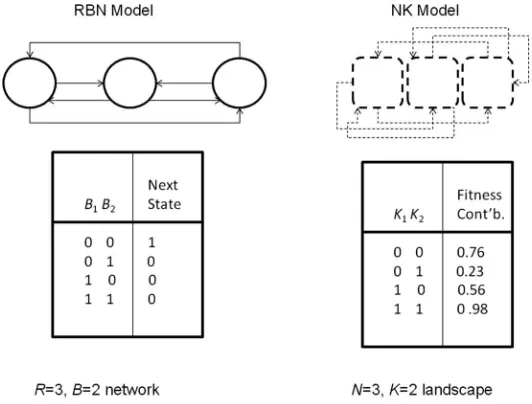
Within the traditional form of RBN—a network ofRnodes, each with a randomly assigned Boolean update function andBdirected connections randomly assigned from other nodes in the network— all updates are synchronous and based upon the current state of thoseB nodes (Figure 1). Hence those B nodes are seen to have a regulatory effect upon the given node, specified by the given Boolean function attributed to it. Since they have a finite number of possible states and they are deterministic, such networks eventually fall into an attractor. It is well established that the value of

Baffects the emergent behavior of RBNs wherein attractors typically contain an increasing number of states with increasingB(see [13] for an overview). Three regimes of behavior exist: ordered when B =1, with attractors consisting of one or a few states; chaotic when B ≥ 3, with a very large number of states per attractor; and a critical regime around B =2, where similar states lie on trajectories that tend to neither diverge nor converge (see [8] for formal analysis).

Kauffman and Levin [14] introduced the NK model to allow the systematic study of various aspects of fitness landscapes (see [13] for an overview). In the standard model an individual is rep-resented by a set ofN(binary) genes or traits, each of which depends upon its own value and that of K randomly chosen others in the individual (Figure 1). Thus, increasingK with respect toN increases the epistasis. This increases the ruggedness of the fitness landscapes by increasing the number of fitness peaks. The NK model assumes all epistatic interactions are so complex that it is only appropriate to assign (uniform) random values to their effects on fitness. Therefore, for each of the possibleKinteractions, a table of 2K+1fitnesses is created, with all entries in the range 0.0 to 1.0, such that there is one fitness value for each combination of traits. The fitness contribution of each trait is found from its individual table. These fitnesses are then summed and normalized byN to give the selective fitness of the individual. Exhaustive search of NK landscapes [22] suggests three general classes exist: unimodal when K=0; uncorrelated, multi-peaked whenK> 3; and a critical regime around 0 <K< 4, where multiple peaks are correlated.

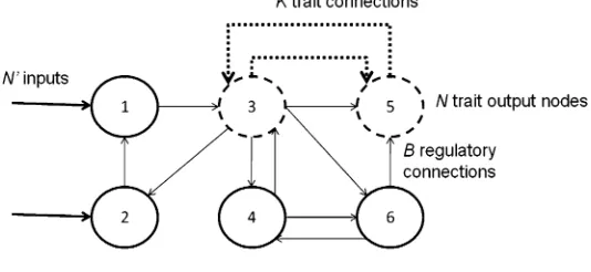
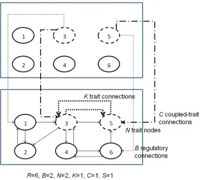
As shown in Figure 2, in the RBNK modelNnodes in the RBN are chosen asoutputs, that is, their state determines fitness using the NK model. The combination of the RBN and NK models enables a systematic exploration of the relationship between phenotypic traits and the genetic regulatory network by which they are produced. It was previously shown how achievable fitness decreases with increasingB, how increasingNwith respect toR decreases achievable fitness, and how R can be decreased without detriment to achievable fitness for low B [3]. Hence the NK element creates a tunable component to the overall fitness landscape with behavior (potentially) influenced by the environment.

Kauffman and Johnsen [15] presented a coevolutionary variant of the NK model—the NKCS model. Here each node (gene) is coupled toKothers locally and toC(also randomly chosen) within each of theSother individuals with which it interacts or is dependent upon in some way. It is shown that asCincreases, the mean performance drops and the time taken to reach an equilibrium point increases, along with an associated decrease in the equilibrium fitness level. That is, adaptive moves made by one partner deform the fitness landscape of its partner(s), with increasing effect for increasing C. As in the NK model, it is again assumed that all intergenome (C) and intragenome (K) interactions are so complex that it is only appropriate to assign random values to their effects on fitness. Therefore for each of the possibleK+CSinteractions, a table of 2K+1+CSfitnesses is created, with all entries in the range 0.0 to 1.0, such that there is one fitness value for each combination of traits. The fitness

Figure 2.Example RBNK model with an equal number of input and output nodes. Dashed lines and nodes indicate where the NK fitness landscape is embedded into the RBN model (refer to Figure 1).

contribution of each gene is found from its individual table. These fitnesses are then summed and normalized byNto give the selective fitness of the total genome (see [13] for an overview).

The RBNK model is easily extended to consider the interaction between multiple GRNs based on the NKCS model—the RBNKCS model [3]. As Figure 3 shows, it is here assumed that the current state of theNtrait nodes of one network provide input to a set ofNinternal nodes in each of its coupled partners, that is, each serves as one of theirBconnections. Similarly, the fitness con-tribution of theNtrait nodes considers not only theKlocal connections, but also theCconnections to itsScoupled partnersʼtrait nodes.

3 Structural Dynamism

In the aforementioned initial study of mobile DNA in RBN [2], structural dynamism was seen as a consequence of the actions of DNA transposons. That is, the cutting and pasting of segments of DNA was seen as causing a change in the connectivity structure of the GRN. Here nodes were extended to (potentially) include a second set ofB0connections to defined nodes. Each such dynamic node also performed an assigned rewiring function based upon the current state of theB0nodes, as shown in Figure 4. Hence on each cycle, each node updates its state based upon the current state of theBnodes it is connected to, using the Boolean logic function assigned to it in the standard way. Then, if that node is also structurally dynamic, thoseBconnections are altered according to the current state of theB0nodes it is connected to, using its rewiring table. The moving of theBconnections of a given node via the states of theB0nodes is therefore seen as an abstraction of one or more of the possible effects of a mobile element as discussed above, triggered by one or more of theB0 nodes, causing a change in the regulatory network, which affects the given node. For simplicity, the number of regulatory connections (B) is assumed to be the same as for rewiring (B0).

As in [13], a genetic hillclimber was considered in [2], and is here. Each RBN is represented as a list to define, for each node, the start state, Boolean function,Bconnection IDs,B0connection IDs,

and connection change table entries, and whether it is a dynamic node or not. Mutation can therefore either (with equal probability): alter the Boolean function of a randomly chosen node; alter a randomly chosenB connection (used as the initial connectivity if a dynamic node); alter a node start state; turn a node into or out of being a dynamic rewiring node; alter one of the rewiring entries in the lookup table if it is a dynamic node; or alter a randomly chosenB0 connection, again only if it is a dynamic node. In the RBNK model a single fitness evaluation of a given GRN was ascertained by updating each node for 100 cycles from the genome-defined start states. At each update cycle, the value of each of theNtrait nodes in the GRN is used to calculate fitness on the given NK landscape. The final fitness assigned to the GRN is the average over 100 such updates. A mutated GRN becomes the parent for the next generation if its fitness is higher than that of the original. In the case of fitness ties, the number of dynamic nodes is considered and the smaller number favored, the decision being arbitrary upon a further tie. Hence there is a slight selective pressure against structural dynamism.

Using the RBNK model in this way, it was shown that forB< 3, starting with no dynamic nodes, around 5% of nodes became dynamic in a nonstationary environment but that dynamic nodes were not incorporated in a stationary environment [2]. The nonstationary case was created by applying a second input string and using a second NK fitness landscape for the latter half of an evaluation. Analy-sis of the rewiring behavior in the low-Bcases showed that the dynamic nodes typically fired foronly the first few update cycles after both initialization and the switch in input halfway through the life cycle. Thus it appears that in low-connectivity networksthe evolutionary process was exploiting structural dynamism to help shape the attractor space of the RBN so that high fitness was reliably reached, depending upon the environmental input and GRN state. This nonstationary case was somewhat motivated by the growing number of examples of environmentally triggered—typically under stress conditions—genomic rearrangements found in a wide variety of organisms (e.g., see [19]).

Figure 4.Example RBN with structural dynamism as in [2]. The lookup table and connections for node 3 are shown in an

R=6,B=2 network. Nodes capable of rewiring haveB0extra structure regulation connections into the network (dashed arrows) and use the states of those nodes to alter the standardBtranscription regulation connections (solid arrows) on the next update cycle (B0=2). Thus in the RBN shown, node 3 is a dynamic node and uses nodes 1 and 2 to determine any structural changes. At update stept, node 3 is shown using the states of nodes 4 and 5 to determine its state for the next cycle. Assuming all nodes are at state 0, the given node above would transit to state 1 for the next cycle and source itsBinputs from nodes 6 and 3 on that subsequent cycle, as defined in the first row of the table shown. A DNA transposon-like mediated change in the regulation network is said to have occurred and the genome rewritten— theBsource connection IDs are altered.

As briefly noted at the end of [2], the structural dynamism can be defined in a position-relative way instead of the explicit addressing form shown in Figure 3. That is, the entries in the columns for theB0 nodes become movements in a range relative to their current connection IDs, for example, using a range ±5 nodes, stopping at either end of the genome. The results were largely unchanged using this approach, one that may be seen as more akin to a DNA transposon excising itself at a given location and inserting itself at the next available appropriate position along the genome— which might be viewed as being a less specific insertion process than that shown in Figure 3. Though not previously reported, analysis of the underlying behavior indicates that the dynamic nodes typically experience continual rewiring during execution, usually moving among a finite set of connections as the RBN moves through its (deterministic) attractor. That is, the rewiring con-nections were typically made to nodes that alter their state within the attractor of the network, whereas with the previous mechanism the rewiring connections were typically made to nodes that do not alter their state within the resulting attractor. Since no marked difference in fitness between these mechanisms was previously observed, node-relative dynamism is used here.

4 Multicellularity

The role of mobile DNA in multicellular natural systems is only just beginning to be explored. There is some evidence that retrotransposons are active in embryogenesis to create somatic variation (e.g., [10]), although the known effects are often linked to disease. More significantly, it is clear that retro-transposons create diversity during neurogenesis within human brain areas such as the hippocampus (e.g., [6]).

The case of two interacting cells has previously been explored with the RBNKCS model, where one is the daughter (clone) of the other, that is,S=1 ([3, 4], after [1]). The (reproducing) mother cell is updated through one cycle and then both update in turn for 100 cycles, thereby introducing some asymmetry in GRN states into the model, with the mother receiving the average fitness of the two cells. HereR=100,N=10, and the results are averaged over 100 runs—10 runs on each of 10 landscapes per parameter configuration—for 30,000 generations. As in [3], 0 <B≤5, 0≤K< 5, and 0 <C≤5 are used.

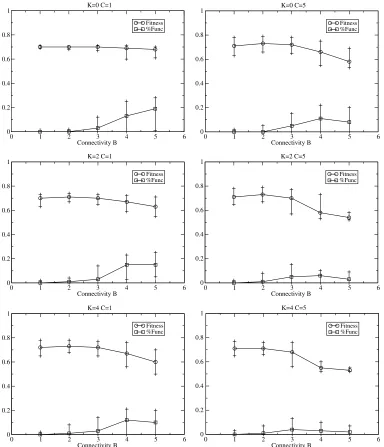
Figure 5 shows examples of typical evolutionary behavior over time for such two-cell systems for varying degrees of intercellular couplingC. As can be seen, dynamism is selected for to around 1% on average in the case of critical connectivity (B=2) shown. Figure 6 shows further examples of various parameter combinations after 30,000 generations of evolution. ForB=1 dynamism is not selected for on average, regardless of the value ofC. Recall that such networks typically exhibit a point or small attractor, and hence the GRNs of the two cells exist in relatively static environ-ments. Dynamism is selected for in all otherBcases. Analysis of the underlying dynamic connection

behavior is as reported above. Fitness drops significantly for higherB, as seen in the RBNK model with and without the structural dynamism previously used [2], and also in the RBNKCS model of multicellularity with and without that form of structural dynamism [3, 4].

5 Functional Dynamism

Probabilistic RBNs (e.g., see [20]) allow for a change in node function within a given set according to a fixed distribution. It has long been noted (e.g., see [12]) that a bias in the Boolean function space of

Figure 6.Performance of the structurally dynamic RBN in the two-cell case, after 30,000 generations. Error bars show min and max values in all graphs. The percentage of nodes that are structurally dynamic (%Conn) is scaled 0–1, as is fitness.

the traditional RBN—that is, a deviation from the expected average probabilityPof 0.5 for either state as the output—reduces the number of attractors and their size for a given number of nodes and connectivity. Canalizing Boolean node functions can have a similar effect due to their reduced sensitivity to input states (e.g., see [13]). Following the node-relative adjustment scheme used for connectivity, a deterministic context-sensitive form of dynamic node can be defined that incremen-tally alters the number of 0s or 1s in the Boolean function table for that node, as shown in Figure 7. Hence on each cycle, each node updates its state based upon the current state of theBnodes it is connected to using the Boolean logic function assigned to it in the standard way. Then, if that node is also functionally dynamic, the node function is altered according to the current state of the B0 nodes it is connected to. Entries in the B0 columns can now be either 0 or 1. A nodeʼs Boolean logic function is stored as a binary string of 2Bbits. The first bit in that logic function table that is not the same as the entry in the dynamic table indexed by the current state of the B0 connections is flipped. In this way, node function can be varied in an incremental way, based upon the current internal and external state of the RBN, here seen as capturing different aspects of mobile DNA than the structural dynamism.

Figure 8 shows that the typical behavior for functional dynamism is generally the same as for structural dynamism for lowB. However, in contrast to the single-cell scenarios explored previously [3] and the structurally dynamic scenarios in [2] and above, the difference in fitness reached between the low- and high-B(>3) cases is not always significant for low inter-cell coupling (T-test,p< 0.05), particularly when the underlying fitness landscape is correlated, that is,K< 4. This effect disappears when the degree of coupling between the two cells increases. That is, for lowC, evolution appears able to exploit functional dynamism effectively for highB. Analysis of the relatively high levels of functionally dynamic nodes indicates similar constant cyclic adjustment within an attractor as seen

Figure 7.Example RBN with functional dynamism. The lookup table and connections for node 3 are shown in anR=6,

for the related form of structural dynamism. Such nodes do not appear to be driven to“saturation” wherein they are either constantly on or constantly off and thereby, perhaps, mitigating the effects of high connectivity in a direct way: Analysis of the resultingP-values of dynamic nodes gives an average of around 0.5, although with high variance (typically 0.2), indicating some specific tuning of attractors via the alteration ofPwithin specific nodes (not shown). Thus it appears that functional dynamism is used to alter the attractor space of the two cells so that their inherently chaotic behavior is mutually contained and hence relatively high fitness levels are achieved, that is, cooperative be-havior emerges. This result has been further explored in the single-cell case, and, as Figure 9 shows, the same fitness benefit is seen even on traditional stationary fitness landscapes where structural

Figure 8.Performance of the functionally dynamic RBN in the two-cell case, after 30,000 generations. The percentage of nodes that are functionally dynamic (%Func ) is scaled 0–1, as is fitness.

dynamism is not selected for. Therefore,functional dynamism appears to give evolution the general ability to tolerate a wide range of levels of gene interconnectivity.

6 Combined Dynamism

The two previous transposon-inspired mechanisms can be combined so that dynamic nodes may be either structurally or functionally variable (in principle, a node could be dynamic in both ways, but

Figure 9.Example performance of the single-cell case with functional dynamism on a stationary landscape. The percent-age of nodes that are functionally dynamic (%Func ) is scaled 0–1, as is fitness.

that has not been explored here). Figure 10 shows example behavior of the RBN with the combined dynamism. As can be seen, dynamic nodes typically represent similar percentages to those in the functional-only case, with analysis indicating more functional nodes for highB, as expected (not shown). Neither form of dynamism is preferred in the high-Ccases, again as predicted from the previous results with only one form possible.

In the above experiments an offspringʼs nodes were initialized according to their genome specifi-cation as in the previous work on evolving RBNs, regardless of the final connectivity pattern and/or node functionality of the parent due to the effects of any dynamic nodes it contained. That is, genomic rearrangements were not inherited. However, it has long been argued that transposon-mediated changes are a principal source of heritable variation in natural evolution (e.g., [18]). Figure 11 shows the evolu-tionary behavior of the dynamic RBN when the parentʼs final network structure, functionality, and node states are inherited by the offspring. The very first RBNs are assigned random connectivity, functions, and node start states. The results indicate there is no significant change in fitness or the percentage of dynamic nodes (T-test,p≥0.05) from the previous version for allBandKcombinations used (compare with Figure 10). That is, there is no significant change in the evolutionary process when the effects of the transposable elements are inheritable, as also reported in [2].

Of course, one of the main benefits of multicellularity is the potential for functional differentiation between cells. Figure 12 shows results where some form of differentiation in the daughterʼs role is expected such that it exists on a different NKCS landscape from the mother, again with inherited struc-tural changes. The results indicate that forB=1, regardless ofKandC, dynamism is selected for in around 1% of nodes on average. ForB=2 there is on average around 4% of dynamic nodes per GRN

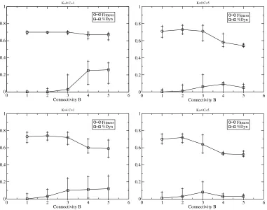
Figure 11.Performance of the fully dynamic RBN where offspring inherit the genomic changes made during the life cycle of the parent, after 30,000 generations. The percentage of nodes that are either structurally or functionally dynamic (%Dyn) is scaled 0–1, as is fitness.

over variousKandC. This is a statistically significant increase (T-test,p< 0.05) in dynamism compared to the equivalent homogeneous case above. Again, there are roughly equal amounts of structural and functional dynamism for lowB, and slightly more functional dynamism for highB. The ability of evolution to exploit dynamism in the high-B and low-Ccases typically remains, particularly when K< 4. Hencecell differentiation is facilitated through the structural and functional dynamism mechanisms.

7 Coevolution

The case of two coevolving GRNs has previously been explored using the RBNKCS model, with each evolved separately on its own NKCS fitness landscape for their Nexternal traits [3]. Each network again updates in turn for 100 cycles, as above. The fitness of one network is then ascertained, and an evolutionary generation for that network is undertaken. The mutated network is evaluated with the same partner—structurally and functionally reset—as the original, and it becomes the parent under the same criteria as used above. Then the second population network is evaluated with that network, before a mutated form is created and evaluated against the same partner. Again, it is adopted if it is fitter or has fewer dynamic nodes. One generation is said to have occurred when all four steps have been taken. Due to the symmetry of the simulations, only the fitness of one population is shown.

Figure 13 shows the performance of the inherited, combined-dynamism RBN. It can be seen that forB=1, regardless ofK, dynamism is not selected for with lowCbut is selected for in around 2% of nodes on average for highC. ForB=2 there is on average around 2% of dynamic nodes per GRN over variousKfor lowCand 10% for highC. There is typically an increase in the amount of dynamism for

the sameBandKbetweenC=1 andC=5 here, although with high variance. Again, there are roughly equal amounts of structural and functional dynamism. In these cases, unlike the multicellular case above, by constantly varying structure and function, the coupled networks are exhibiting uncooperative behavior: The ability to dynamically alter the attractor space appears to make it easier for the coupled networks to compensate for or cause changes in behavior. The ability of evolution to exploit dynamism in the high-Bcases is seen again; however, this behavior, unlike in the multicellular scenario, is not

Figure 13.Performance of the fully dynamic RBN coevolved against another, after 30,000 generations. The percentage of nodes that are either structurally or functionally dynamic (%Dyn) is scaled 0–1, as is fitness.

sensitive toC. The amount of dynamism rises to around 20% for lowCand increases further for highC, although the fitness levels become increasingly variable.

Figure 14 shows example single runs of these systems, indicating how the degree of dynamic nodes varies temporally depending upon the underlying coevolutionary behavior: During periods of stasis, dynamism is selected against, but it rises dramatically during periods of readaptation to a change in the partner species. This automatic adjustment in the rate of change of a genome, driven by current evolutionary behavior, is somewhat reminiscent of that displayed by self-adaptive mutation operators in evolutionary computing in nonstationary environments (e.g., [9]).

8 Conclusions

The evolutionary significance of mobile DNA is becoming increasingly clear (e.g., [19]). This article has explored the use of novel mechanisms based upon transposons within an extended version of a well-known abstract model of coupled GRNs. Building upon recent results, it has been shown that simple structural and functional dynamism are positively selected for in environments containing more than one GRN, either in isolation or when both mechanisms are available simultaneously. Moreover, any genomic rearrangements occurring during a parentʼs life cycle can be inherited by the offspring without detriment. Perhaps most significantly, functional dynamism is found to enable evolution to tolerate high levels of gene connectivity in single and coupled GRN scenarios.

There is a growing body of work within evolutionary computation that explores representations more closely analogous to those seen in nature, that is, artificial genetic regulatory networks (e.g., see [3] for an overview). Adoption of these relatively generic representations creates the opportunity to exploit new search mechanisms based upon the more recent discoveries of microbiology. Namely, molecular biologists have identified a variety of mechanisms through which changes in DNA occur in natural regulatory networks in ways other than the processes that inspired the traditional search heuristics of evolutionary computation: Specific biochemical processes generate novelty through tar-geted DNA restructuring based upon the internal and external state of a GRNduringthe organismal life cycle. This article has presented two new mechanisms for use within artificial genetic regulatory networks, which may prove useful in the solution of complex problems.

Further consideration of mobile DNA suggests a number of extensions to this work in the near future, particularly the use of retrotransposon-like copying to enable new mechanisms for changing the size of the GRN (see [3]). Approaches drawing upon that recently presented by Smith et al. [21] would seem appropriate, for example. Future work should also consider the use of transposon-inspired mechanisms within other GRN representations, explore whether these results also hold for asynchronous GRN updating schemes (after [2]), and determine whether the general results also appear to be true for much larger coevolutionary systems, that is, for S≫1 (see [5] for an initial study).

References

1. Bull, L. (1999). On the evolution of multicellularity and eusociality.Artificial Life,5(1), 1–15.

2. Bull, L. (2012). Evolving Boolean networks with structural dynamism.Artificial Life,18(4), 385–398.

3. Bull, L. (2012). Evolving Boolean networks on tunable fitness landscapes.IEEE Transactions on Evolutionary Computation,16(6), 817–828.

4. Bull, L. (in press). Consideration of mobile DNA: New forms of artificial genetic regulatory networks.

Natural Computing,12(4), 443–452.

5. Bull, L., & Adamatzky, A. (2013). Evolving gene regulatory networks with mobile DNA mechanisms. In Y. Jin & S. Thomas (Eds.),Proceedings of the UK Workshop on Computational Intelligence(pp. 1–7). Piscataway, NJ: IEEE Press.

7. Craig, N., Craigie, R., Gellert, M., & Lambowitz, A. M. (2002).Mobile DNA II. Washington: American Society for Microbiology Press.

8. Derrida, B., & Pomeau, Y. (1986). Random networks of automata: A simple annealed approximation.

Europhysics Letters,1, 45–49.

9. Hoffmeister, F., & Back, T. (1992). Genetic self-learning. In F. J. Varela & P. Bourgine (Eds.),

Toward a Practice of Autonomous Systems: Proceedings of the First European Conference on Artificial Life

(pp. 227–235). Cambridge, MA: MIT Press.

10. Kano, H., Godoy, I., Courtney, C., Vetter, M., Gerton, G., Ostertag, E., & Kazazian, H. (2009). L1 retrotransposition occurs mainly in embryogenesis and creates somatic mosaicism.Genes &

Development,23(11), 1303–1312.

11. Kauffman, S. A. (1969). Metabolic stability and epigenesis in randomly constructed genetic nets.

Journal of Theoretical Biology,22, 437–467.

12. Kauffman, S. A. (1984). Emergent properties in random complex automata.Physica D,10, 145.

13. Kauffman, S. A. (1993).The origins of order. Oxford, UK: Oxford University Press.

14. Kauffman, S. A., & Levin, S. (1987). Towards a general theory of adaptive walks on rugged landscapes.

Journal of Theoretical Biology,128, 11–45.

15. Kauffman, S. A., & Johnsen, S. (1992). Coevolution to the edge of chaos: Coupled fitness landscapes, poised states, and coevolutionary avalanches. In C. Langton et al. (Eds.),Artificial Life II(pp. 325–370). Redwood City, CA: Addison-Wesley.

16. Kazazian, H. (2004). Mobile elements: Drivers of genome evolution.Science,303, 1626–1632.

17. McClintock, B. (1987).Discovery and characterization of transposable elements: The collected papers of Barbara

McClintock. New York: Garland.

18. Shapiro, J. (1992). Natural genetic engineering in evolution.Genetica,86, 99–111.

19. Shapiro, J. (2011).Evolution: A view from the 21st century. Upper Saddle River, NJ: FT Press.

20. Shmulevich, I., & Dougherty, E. (2010).Probabilistic Boolean networks: The modeling and control of gene

regulatory networks. Philadelphia: Society for Industrial and Applied Mathematics.

21. Smith, D., Onnela, J.-P., Lee, C., Fricker, M., & Johnson, N. (2011). Network automata: Coupling structure and function in dynamic networks.Advances in Complex Systems,14(3), 317–339.