On the Evolution of Boolean Networks for Computation:
A Guide RNA Mechanism
Larry Bull
University of the West of England
Bristol BS16 1QY, U.K.
Abstract
There is a growing body of work within computational intelligence which explores the use of
representations inspired by the genetic regulatory networks of biological cells. This paper
uses a recently presented abstract, tunable model of such networks to investigate how their
design through simulated evolution is affected through the ability to dynamically re-wire
connectivity. The contextual editing of transcribed RNA by other molecules such that the
form of the final product differs from that specified in the corresponding DNA sequence is
ubiquitous. It is here shown that a guide RNA-inspired editing mechanism can be selected for
under various scenarios.
Introduction
The genetic regulatory networks (GRN) within cells synthesize molecules which both directly and indirectly affect behaviour. That is, within a given GRN, some genes encode for RNA/proteins which have regulatory functions, some which have intra-cellular function, and some which pass through the cell membrane. A growing body of work within computational intelligence, particularly evolutionary computation, is exploring parallel, emergent systems inspired by the natural phenomena. With the aim of enabling the systematic exploration of artificial GRN models, a simple approach to combining them with abstract fitness landscapes has recently been presented [1]. More specifically, random Boolean networks (RBN) [2] were combined with the NK model of fitness landscapes [3]. In the combined form – termed the RBNK model – a simple relationship between the states of N randomly assigned nodes within an RBN is assumed such that their value is used within a given NK fitness landscape of trait dependencies. The approach was also extended to enable consideration of multi-agent coevolutionary and multicellular scenarios using the related NKCS landscapes [4] – termed the RBNKCS model. This paper uses the RBNK and RBNKCS models to explore the evolution of GRN within primarily non-stationary problem spaces, that is, where the underlying features of the task are temporally dynamic.
thereby (typically) altering the structure of the protein specified in the expressed DNA. In this paper, RBNs are extended to include a simple form of RNA editing. The selection of the extra mechanism is explored under various single and multiple cell scenarios. Results indicate guide RNA editing is useful across a wide range of conditions, particularly those with non-stationary fitness landscapes.
There appears to be very little work which considers the role of RNA editing explicitly. After [7], Huang et al. (see [8] for an overview) have explored the use of a stochastic template matching mechanism which either inserts or deletes binary genes for function optimization. They report consistent benefit for dynamic/non-stationary functions in particular. Rohlfshagen and Bullinaria [9] used an RNA editing-inspired scheme as a repair function for multi-constrained knapsack problems. Some formal models of aspects of RNA editing have also been presented (eg, [10]). No previous work with artificial GRN is known.
There is a small amount of prior work exploring the use of simulated evolution to design
GRN and RBN in particular (see [1] for an overview). Van den Broeck and Kawai [11]
explored the use of a simulated annealing-type approach to design feedforward RBN for the
four-bit parity problem. Kauffman [12, p.211] evolved RBN to match a given attractor.
Lemke et al. [13] did the same (see [14] for an overview of work evolving the related
threshold networks to an attractor). The same approach has been used to explore attractor
stability [15] and to model real regulatory network data, eg, see [16] for an example using
probabilistic RBN. Sipper and Ruppin [17] evolved RBNfor the well-known density task and
Bull [18] has evolved RBN ensembles to solve benchmark machine learning problems. RBN
Background
The RBNK Model
Within the traditional form of RBN, a network of R nodes, each with a randomly assigned Boolean update function and B directed connections randomly assigned from other nodes in the network, all update synchronously based upon the current state of those B nodes. Hence those B nodes are seen to have a regulatory effect upon the given node, specified by the given Boolean function attributed to it. Since they have a finite number of possible states and they are deterministic, such networks eventually fall into an attractor. It is well-established that the value of B affects the emergent behaviour of RBN wherein attractors typically contain an increasing number of states with increasing B (see [12] for an overview). Three regimes of behaviour exist: ordered when B=1, with attractors consisting of one or a few states; chaotic when B≥3, with a very large number of states per attractor; and, a critical regime around B=2,
where similar states lie on trajectories that tend to neither diverge nor converge. Note that traditionally the size of an RBN is labelled N, as opposed to R here, and the degree of node connectivity labelled K, as opposed to B here. The change is adopted due to the traditional use of the labels N and K in the NK model of fitness landscapes.
created, with all entries in the range 0.0 to 1.0, such that there is one fitness value for each combination of traits. The fitness contribution of each trait is found from its individual table. These fitnesses are then summed and normalised by N to give the selective fitness of the individual. Three general classes exist: unimodal when K=0; uncorrelated, multi-peaked when K>3; and, a critical regime around 0<K<4, where multiple peaks are correlated.
[Figure 1]
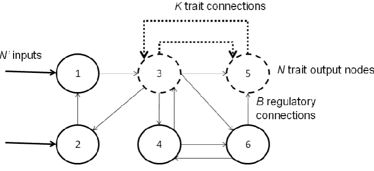
As shown in Figure 1, in the RBNK model N nodes (where R≤N<0) in the RBN are chosen as
outputs/traits, i.e., their state determines fitness using the NK model. The combination of the RBN and NK model enables a systematic exploration of the relationship between phenotypic traits and the genetic regulatory network by which they are produced. It was previously shown how achievable fitness decreases with increasing B, how increasing N with respect to R decreases achievable fitness, and how R can be decreased without detriment to achievable
fitness for low B [1]. In this paper N phenotypic traits are attributed to randomly chosen nodes within the network of Rgenetic loci, with environmental inputs applied to the first N’ loci (Figure 1); input nodes and trait/output nodes are not necessarily disjoint. Hence the NK element creates a tunable component to the overall fitness landscape with behaviour (potentially) influenced by the environment. For simplicity, N’=N here.
The RBNKCS Model
range 0.0 to 1.0, such that there is one fitness value for each combination of traits. The fitness contribution of each gene is found from its individual table. These fitnesses are then summed and normalised by N to give the selective fitness of the total genome (see [12] for an overview). It is shown that as C increases, mean fitness drops and the time taken to reach an equilibrium point increases, along with an associated decrease in the equilibrium fitness level. That is, adaptive moves made by one partner deform the fitness landscape of its partner(s), with increasing effect for increasing C. As in the NK model, it is again assumed all intergenome (C) and intragenome (K) interactions are so complex that it is only appropriate to assign random values to their effects on fitness.
[Figure 2]
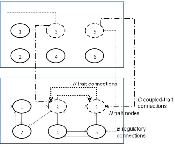
The RBNK model is easily extended to consider the interaction between multiple GRN based on the NKCS model – the RBNKCS model. As Figure 2 shows, it is here assumed that the current state of the N trait nodes of one network provide input to a set of N internal nodes in each of its coupled partners, i.e., each serving as one of their B connections. Similarly, the fitness contribution of the N trait nodes considers not only the K local connections but also the C connections to its S coupled partners’ trait nodes. The GRN update alternately.
RNA Editing in the RBNK(CS) Model
gRNA
table for the B’ connections where the node is on/expressed. The list is the same size as the
out-degree of the node (range [0, R*B]). This is seen as introducing a non-coding RNA associated with the protein expressed by the given node. RNA editing causes a change in the connectivity of the RBN which lasts for one update cycle.
[Figure 3]
On each traditional RBN update cycle, the connectivity of the network is initially assumed (reset) to be that originally determined by evolution. Then, for each node which has an associated guide RNA, a check is made to see if the node’s transcription state was set to on (’1’) on the last update step and if its associated RNA has been activated (‘1’) since the last
time this occurred. If so, the out-connections for that node are altered to those in the corresponding table entry for the current state of the B’ connection nodes (Figure 3). If a node
RBNK Experimentation
For simplicity with respect to the underlying evolutionary search process, a genetic hill-climber is considered here, as in [1]. Each RBN is represented as a list to define each node’s start state, Boolean function for transcription, B connection ids, B’ connection ids, Boolean function for RNA editing, re-connectivity entries under RNA editing, and whether it is an RNA edited node or not. Mutation can therefore either (with equal probability): alter the Boolean transcription function of a randomly chosen node; alter a randomly chosen B connection; alter a node start state; turn a node into or out of being RNA editable; alter one of the re-connection entries if it is an editable node; or, alter a randomly chosen B’ connection, again only if it is an editable node. A single fitness evaluation of a given GRN is ascertained by updating each node for 100 cycles from the genome defined start states. An input string of N’ 0’s is applied on every cycle here. At each update cycle, the value of each of the N trait
nodes in the GRN is used to calculate fitness on the given NK landscape. The final fitness assigned to the GRN is the average over 100 such updates here. A mutated GRN becomes the parent for the next generation if its fitness is higher than that of the original. In the case of fitness ties the number of RNA editable nodes is considered, with the smaller number favoured, the decision being arbitrary upon a further tie. Hence there is a slight selective pressure against RNA editing. Here R=100, N=10 and results are averaged over 100 runs - 10
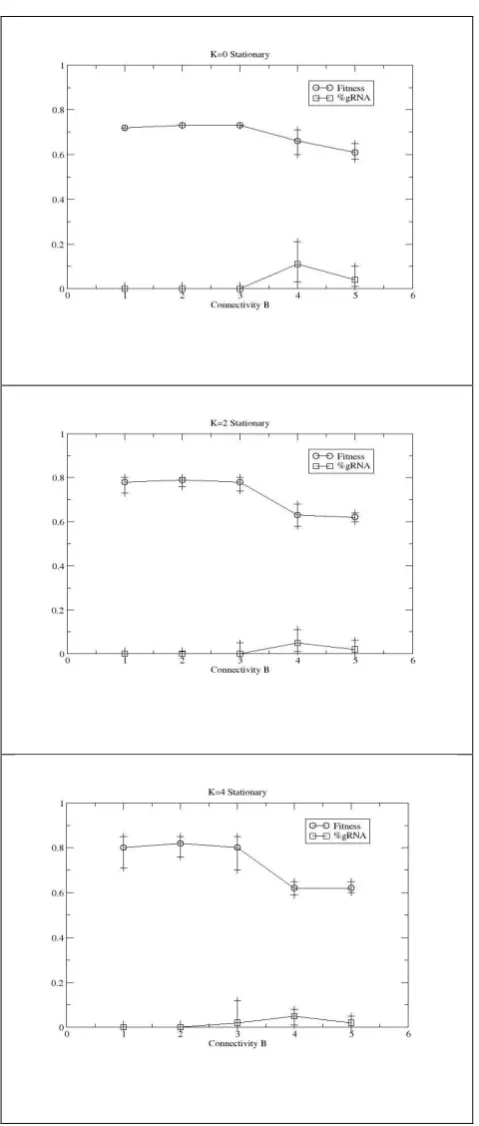
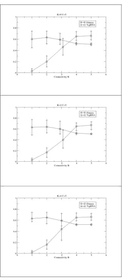
runs on each of 10 landscapes per parameter configuration - for 50,000 generations, 0<B≤5 and 0≤K≤5 are used. As Figure 4 shows, regardless of K, RNA editing is selected for in all
Since it is known such highly connected networks typically exhibit chaotic dynamics [12] and they are subsequently difficult to evolve [1], it might be surmised that the RNA editing is not performing a functional role, rather it is maintained under drift/neutral processes. As noted above, RNA editing alters the out-connections of a given node and hence a potential consequence is the alteration in the number of connections into a given node. In particular, given the seemingly positive selection of editing in the high B cases in Figure 4 it might be assumed that the mechanism’s ability to effectively reduce a node’s B is all that is being
selected for since fitness drops with increasing B. Experiments (not shown) in which the out-connection table entries are randomly re-created in the offspring indicate a significant (T-test, p<0.05) drop in fitness in all cases where editing is selected for and hence evolution does
appear to be shaping suitable, dynamic behaviour through the editing mechanism. Although some editing nodes are also almost certainly there due to drift/neutral processes.
[Figure 4]
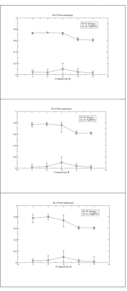
Following [8], Figure 5 shows how RNA editing is selected for under all conditions when the underlying fitness landscape changes halfway through the lifecycle; an input of all 1’s is
applied on update cycle 50 and fitness contributions are calculated over a second NK landscape. Analysis of typical behaviour in the low B cases shows that one or two nodes use editing either up to or after the point of change. That is, the editing is used to make small changes to the network topology to compensate for the disruption in the environment; the RNA editing has an active (context sensitive) role in the cyclic behaviour of the networks. These general results were also found for other values of R, eg, R=200 (not shown).
RBNKCS Experimentation
Heterogeneous cells
The case of two coevolving GRN has previously been explored using the RBNKCS model, each evolved separately on their own NKCS fitness landscape for their N external traits [1]. Each network updates in turn for 100 cycles. The fitness of one network is then ascertained and an evolutionary generation for that network is undertaken. The mutated network is evaluated with the same partner as the original and it becomes the parent under the same criteria as used above. Then the second species network is evaluated with that network, before a mutated form is created and evaluated against the same partner. One generation is said to have occurred when all four steps have been undertaken. Only the fitness of the species with the potential to exploit RNA editing is shown here. This general scenario is potentially of interest given the proposed role of RNA editing by cells against viruses [20], for example.
[Figure 6]
drift/neutral processes within such poorly evolving systems. The exact ways in which the editing is used in the low B cases is hard to establish. Figure 7 shows how the same general trends occur for higher levels of coupling between the two, i.e., C=5. It can be noted that some level of RNA editing is now seen when B=1.
[Figure 7]
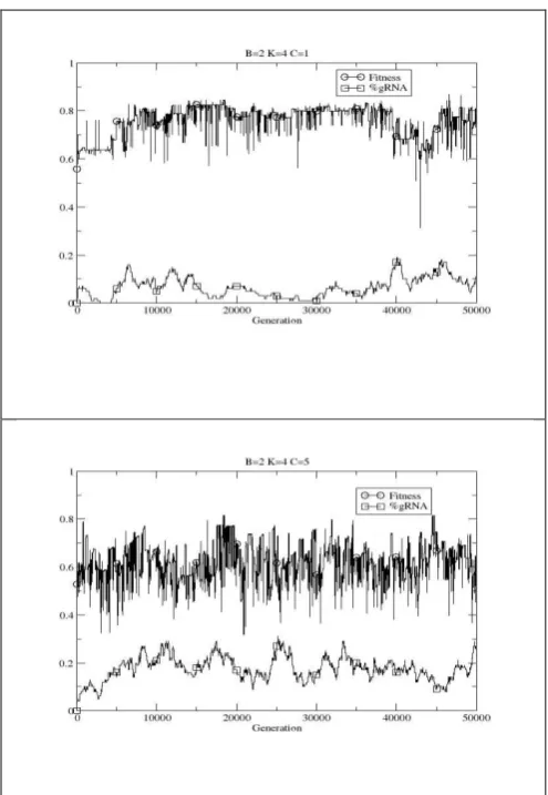
Analysis of how the percentage of RNA editing nodes varies over time shows relatively stable behaviour in the RBNK model (not shown). Figure 8 shows example runs of how this is not the case in the RBNKCS model, rather the percentage varies over time. Indeed, it appears there is a rough correlation between periods of coevolutionary stasis with regards to fitness and a decrease in the percentage of RNA editing nodes, and vice versa, for lower values of C.
[Figure 8]
Homogeneous cells
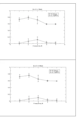
[Figure 9]
Figure 9 shows examples of how the degree of adoption of the RNA editing in such cases is almost identical to that seen in the non-stationary single cell cases above. That is, it is seen for all B at relatively low levels. Similar results (not shown) are seen when task differentiation is not assumed between the cells. Again, understanding how the mechanism is used in the coupled cells is non-trivial.
Discussion
RNA editing appears to serve many roles [6], including (organelle) mutation repair and defence against viruses. From a regulatory network perspective, editing such as that provided by guide RNA enables context sensitive structural dynamism. This (temporary) re-wiring of the underlying network topology provides a further layer of regulation. The results in this paper suggest that the mechanism will be selected for across a wide variety of conditions, particularly non-stationary and multiple celled scenarios. The correlations between such conditions and practical network domains where time-varying graphs are often applied (eg, [23]), remains to be explored. Results here also indicate selection in high connectivity cases. It can be noted that within natural GRN genes have low connectivity on average (eg, [24]), as RBN predict, but a number of high connectivity “hub” genes perform significant roles (eg,
see [25]). The results here suggest RNA editing may help facilitate such structures.
References
1. Bull, L. (2012). Evolving Boolean networks on tunable fitness landscapes. IEEE Transactions on Evolutionary Computation, 16(6): 817-828.
2. Kauffman, S. A. (1969). Metabolic stability and epigenesis in randomly constructed genetic nets. Journal of Theoretical Biology, 22:437-467.
3. Kauffman, S.A. & Levin, S. (1987). Towards a general theory of adaptive walks on rugged landscapes. Journal of Theoretical Biology, 128: 11-45.
4. Kauffman, S.A. and Johnsen, S. (1991). Coevolution to the edge of chaos: Coupled fitness landscapes, poised states, and coevolutionary avalanches. In Langton, C., et al., editors, Artificial Life II, pages 325-370. Addison-Wesley, MA.
5. Maas, S. (Ed.)(2013). RNA editing: Current research and Future Trends. Caister Academic Press, Norfolk.
6. Gray, M. (21012). Evolutionary origin of RNA editing. Biochemistry, 51: 5235-5242.
8. Huang, C-F., Kaur, J., Maguitman, A. and Rocha, L.M. (2007). Agent-based model of genotype editing. Evolutionary Computation, 15(3): 253-289.
9. Rohlfshagen, P. and Bullinaria, J.A. (2006). An exonic genetic algorithm with RNA editing inspired repair function for the multiple knapsack problem. In Proceedings of the UK Workshop on Computational Intelligence (UKCI 2006), pages 17-24. Springer,
Berlin.
10.Liu, T. and Bundschuh, R. (2005). Model for codon position bias in RNA editing. Phys. Rev. Lett., 95, 088101.
11.Van den Broeck, C. and Kawai, R. (1990). Learning in feedforward Boolean networks. Physical Review A 42: 6210-6218.
12.Kauffman, S.A. (1993). The origins of order. Oxford University Press, Oxford.
13.Lemke, N., Mombach, J. and Bodmann, B. (2001). A numerical investigation of adaptation in populations of random Boolean networks. Physica A 301: 589–600.
14.Bornholdt, S. (2001). Modeling genetic networks and their evolution: A complex dynamical systems perspective. Biol. Chem. 382: 1289 – 1299.
16.Tan, P. and Tay, J. (2006). Evolving Boolean networks to find intervention points in dengue pathogenesis. In GECCO-2006: Proceedings of the Genetic and Evolutionary Computation Conference. Springer, pp307-308.
17.Sipper, M. and Ruppin, E. (1997). Co-evolving architectures for cellular machines. Physica D (99): 428-441.
18.Bull, L. (2009). On dynamical genetic programming: Simple Boolean networks in learning classifier systems. International Journal of Parallel, Emergent and Distributed Systems 24(5): 421-442.
19.Goudarzi, A., Teuscher, C., Gulbahce, N. and Rohlf, T. (2012). Emergent criticality through adaptive information processing in Boolean networks. Phys. Rev. Letts. 108(12): 128702.
20.Grivell, L. (1993). Plant mitochondria 1993 – a personal overview. In Brennicke, A. and Kuck, U., editors, Plant Mitochondria, pages 1–14. VCH Verlagsgesellschaft, Weinheim.
21.Burns, C., Chu, H., Rueter, S., Hutchinson, L., Canton, H., Sanders-Bush, E. and Emerson, R. (1997). Regulation of serotonin-2C receptor G-protein coupling by RNA editing. Nature, 387:303-308.
23.Casteigts, A., Flocchini, P., Quattrociocchi, W. and Santoro, N. (2012). Time-varying graphs and dynamic networks. International Journal of Parallel, Emergent and Distributed Systems 27(5): 387-408.
24.Leclerc, R. (2008). Survival of the sparsest. Molecular Systems Biology, 4: 213-216.
Figure 1: Example RBNK model with an equal number of input and output nodes. Dashed lines and nodes indicate
Figure3: Example RBN with RNA editing. The look-up table and connections for node 3 only are shown for clarity.
Figure 4: Evolutionary performance of RBN augmented with an RNA editing mechanism, after 50,000 generations.
Figure 5: Evolutionary performance of RBN augmented with an RNA editing mechanism, after 50,000 generations,
Figure 6: Performance of the augmented RBN coevolved against another, after 50,000 generations. The percentage
Figure 7: Performance of the augmented RBN coevolved against another, after 50,000 generations, for a high
[image:23.595.174.424.63.633.2]Figure 8: Example single runs of the coevolutionary case showing how editing is exploited to varying degrees
[image:24.595.174.422.97.456.2]Figure 9: Example performance in the two-celled case, after 50,000 generations. The percentage of nodes which use