A Maximum Entropy Inspired Parser

(1)

A M a x i m u m - E n t r o p y - I n s p i r e d

P a r s e r *

E u g e n e Charniak

B r o w n L a b o r a t o r y for L i n g u i s t i c I n f o r m a t i o n P r o c e s s i n g D e p a r t m e n t of C o m p u t e r Science

B r o w n University, B o x 1910, P r o v i d e n c e , R I 02912 e c @ c s . b r o w n . e d u

A b s t r a c t

We present a new parser for parsing down to Penn tree-bank style parse trees t h a t achieves 90.1% average precision/recall for sentences of length 40 and less, and 89.5% for sentences of length 100 and less when trMned and tested on the previously established [5,9,10,15,17] "standard" sections of the Wall Street Journal tree- bank. This represents a 13% decrease in error rate over the best single-parser results on this corpus [9]. The major technical innovation is tire use of a "ma~ximum-entropy-inspired" model for conditioning and smoothing t h a t let us successfully to test and combine many different conditioning events. We also present some partial results showing the effects of different conditioning information, including a surpris- ing 2% improvement due to guessing the lexical head's pre-terminal before guessing the lexical head.

1

I n t r o d u c t i o n

We present a new parser for parsing down to Penn tree-bank style parse trees [16] t h a t achieves 90.1~ average precision/recall for sentences of length < 40, and 89.5% for sentences of length < 100, when trained and tested on the previously established [5,9,10,15,17] "standard" sections of the Wall Street Journal tree-bank. This represents a 13% decrease in error rate over the best single-parser results on this corpus [9]. Following [5,10], our parser is based upon a probabilistic generative model. T h a t is, for all sentences s and MI parses 7r, the parser assigns a probability

p(s,

~) = p(Tr), the equality holding when we restrict consideration to ~r whose yield

* This research was supported in part by NSF grant LIS SBR 9720368. T h e author would like to thank Mark

Johnson and all the rest of the Brown Laboratory for Linguistic Information Processing.

is s. Then for any s the parser returns the parse 7r t h a t maximizes this probability. T h a t is, the parser implements the function

arg. a= p( I

=

= arg

maxTrp(lr).

W h a t fundamentally distinguishes probabilistic generative parsers is how they c o m p u t e p(~r), and it is to t h a t topic we t u r n next.

2

T h e G e n e r a t i v e M o d e l

The model assigns a probability to a parse by a top-down process of considering each constituent c in ~r and for each c first guessing the pre-terminal of

c, t(c) (t

for "tag"), then the lexical head of

c, h(c),

and then the expansion of c into further constituents

c(c).

T h u s the probability of a parse is given by the equation

1"I P(t(c) l l(c),H(c))

cE;¢

.v(h(c) l t(c),l(c),H(c))

.p(e(c) i l(c),t(c),h(c),H(c))

where

l(c)

is the label of c (e.g., whether it is a noun phrase (np), verb-phrase, etc.) and

H(c)is

the relevant history of c - - information outside c t h a t our probability model deems i m p o r t a n t in determining the probability in question. Much of the interesting work is determining what goes into

H(c).

Whenever it is clear to which constituent we are referring we omit the (c) in, e.g.,

h(c).

In this notation the above equation takes the following form:

= 1-[ v(t I l , z ) . v ( h I t,l,H).v(¢ I

cE;¢

(2)

Next we describe how we assign a probability to the expansion e of a constituent. In Sec- tion 5 we present some results in which the possible expansions of a constituent are fixed in advanced by extracting a tree-bank g r a m m a r [3] from the training corpus. T h e m e t h o d t h a t gives the best results, however, uses a Markov g r a m m a r - - a m e t h o d for assigning probabilities to any possible expansion using statistics gathered from the training corpus [6,10,15]. T h e m e t h o d we use follows t h a t of [10]. In this scheme a traditional probabilistic context-free g r a m m a r ( P C F G ) rule can be thought of as con- sisting of a left-hand side with a label

l(e)

drawn from the non-terminal symbols of our g r a m m a r , and a right-hand side t h a t is a sequence of one or more such symbols. (We assume t h a t all terminal symbols are generated by rules of the form

"preterm -+ word'

and we t r e a t these as a special case.) For us the non-terminal symbols are those of the tree-bank, augmented by the symbols aux and auxg, which have been assigned de- terministically to certain auxiliary verbs such as "have" or "having". For each expansion we dis- tinguish one of the right-hand side labels as the "middle" or "head" symbol

M(c). M(c)

is the constituent from which t h e head lexical item h is obtained according to deterministic rules t h a t pick the head of a constituent from a m o n g t h e heads of its children. To the left of M is a sequence of one or more left labels

Li (c)

including the special termination symbol A, which indi- cates t h a t there are no more symbols to the left, and similarly for the labels to the right,

Ri(c).

T h u s an expansion

e(c)

looks like:

1 --~ ALm...L1MRI...RnA.

(2)

T h e expansion is generated by guessing first M , then in order L1 through Lm+t ( = A), and similarly for R1 t h r o u g h R,+~.

In a pure Markov P C F G we are given t h e left-hand side label l and then probabilisticaily generate the right-hand side conditioning on no information other t h a n I and (possibly) previously generated pieces of the right-hand side itself. In t h e simplest of such models, a zero- order Markov g r a m m a r , each label on the right- hand side is generated conditioned only on l - - t h a t is, according to the distributions

p(Li I l),

p(M l I),

and

p(Ri l l).

More generally, one can condition on the m

previously generated labels, t h e r e b y obtaining an m t h - o r d e r M a r k o v g r a m m a r . So, for example, in a second-order Markov P C F G , L2 would be conditioned on L1 and M . In our complete model, of course, the probability of each label in the expansions is also conditioned on other material as specified in Equation 1, e.g.,

p(e I l, t, h, H).

Thus we would use

p(L2 I

L1, M, l, t, h, H ) . Note t h a t t h e As on both ends of the expansion in Expression 2 are conditioned just like any other label in the expansion.

3 M a x i m u m - E n t r o p y - I n s p i r e d

Parsing

T h e m a j o r problem confronting the a u t h o r of a generative parser is w h a t information to use to condition the probabilities required in t h e model, and how to s m o o t h the empirically obtained probabilities to take the sting out of the sparse d a t a problems t h a t are inevitable with even the most m o d e s t conditioning. For example, in a second-order Markov g r a m m a r we conditioned the L2 label according to the distribution

p(L2 I L t , M , I , t , h , H ) .

Also, r e m e m b e r t h a t H is a placeholder for any o t h e r information beyond the constituent e t h a t m a y be useful in assigning c a probability.

In the past few years the m a x i m u m entropy, or log-linear, approach has r e c o m m e n d e d itself to probabilistic model builders for its flexibility and its novel approach to smoothing [1,17]. A complete review of log-linear models is beyond the scope of this paper. Rather, we concentrate on the aspects of these models t h a t most directly influenced the model presented here.

To c o m p u t e a probability in a log-linear model one first defines a set of "features", functions from the space of configurations over which one is trying to c o m p u t e probabilities to integers t h a t denote the n u m b e r of times some p a t t e r n occurs in t h e input. In our work we assume t h a t any f e a t u r e can occur at most once, so features are boolean-valued: 0 if the p a t t e r n does not occur, 1 if it does.

In the parser we f u r t h e r assume t h a t features are chosen from certain feature s c h e m a t a and t h a t every feature is a boolean conjunc- tion of sub-features. For example, in computing the probability of the head's pre-terminal t we might want a f e a t u r e schema f ( t , l) t h a t returns 1 if the observed pre-terminal of c = t and the

(3)

label of c = l, and zero otherwise. This feature is obviously composed of two sub-features, one recognizing

t,

the other 1. If b o t h r e t u r n 1, then the feature r e t u r n s 1.

Now consider computing a conditional probability

p(a I H)

with a set of features f l . . . f j t h a t connect a to t h e history H . In a log-linear model the probability function takes the following form:

1

eXl(a,H)fl(a,H)+...+,km(a,H).fm(a,H)

p(a

I H ) -

Z(H)

(3)

Here the Ai are weights between negative and positive infinity t h a t indicate the relative impor- t a n c e of a feature: the more relevant the feature to the value of the probability, t h e higher t h e ab- solute value of the associated X. T h e function

Z(H),

called the partition function, is a normal- izing c o n s t a n t (for fixed H ) , so t h e probabilities over all a sum to one.

Now for our purposes it is useful to rewrite this as a sequence of multiplicative functions

gi(a,H)

for 0 < i < j :

p(a I H ) = go(a,H)gl(a,H) ...gj(a,H).

(4)

Here

go(a,H) = 1/Z(H)

and

gi(a,H) =

e'~(a'n)f~(a'H).

T h e intuitive idea is t h a t each factor gi is larger t h a n one if the feature in question makes t h e probability m o r e likely, one if the f e a t u r e has no effect, and smaller t h a n one if it makes the probability less likely.

M a x i m u m - e n t r o p y models have two benefits for a parser builder. First, as already implicit in our discussion, factoring the probability compu- tation into a sequence of values corresponding to various 'tfeatures" suggests t h a t the probability model should be easily changeable - - just change the set of features used. This point is emphasized by R a t n a p a r k h i in discussing his parser [17]. Second, and this is a point we have not yet mentioned, t h e features used in these models need have no particular independence of one another. This is useful if one is using a log- linear model for smoothing. T h a t is, suppose we want to c o m p u t e a conditional probability

p(a ] b,c),

but we are not sure t h a t we have enough examples of the conditioning event b, c in the training corpus to ensure t h a t the empirically obtained probability/~(a [ b, c) is accurate. The traditional way to handle this is also to

c o m p u t e / ~ ( a I b), and perhaps iS(a I c) as well, and take some combination of these values as one's best estimate for

p(a I b, c).

This m e t h o d is known as "deleted interpolation" smoothing. In m a x - e n t r o p y models one can simply include features for all three events

fl(a, b, c), f2(a, b),

and f3(a, c) and combine t h e m in t h e model according to Equation 3, or equivalently, Equation 4. T h e fact t h a t t h e features are very far from independent is not a concern.

Now let us note t h a t we can get an equation of exactly t h e same form as E q u a t i o n 4 in the following fashion:

p(alb, c)p(alb, c,d)

p(alb, c , d ) = p ( a l b ) - ~ a l b )

p(alb, c)

(5)

Note t h a t t h e first t e r m of the equation gives a probability based upon little conditioning infor- m a t i o n and t h a t each subsequent t e r m is a num- ber from zero to positive infinity t h a t is greater or smaller t h a n one if t h e new information being considered makes t h e probability greater or smaller t h a n t h e previous estimate.

As it stands, this last equation is p r e t t y much content-free. B u t let us look at how it works for a particular case in our parsing scheme. Con- sider t h e probability distribution for choosing the pre-terminal for t h e head of a constituent. In Equation I we wrote this as

p(t I l, H).

As we discuss in more detail in Section 5, several different features in t h e context surrounding c are useful to include in H : the label, head pre-terminal and head of t h e parent of c (de- noted as

lv, tv, hp),

t h e label of c's left sibling (lb for "before"), and t h e label of t h e grandparent of c (la). T h a t is, we wish to c o m p u t e

p(t I l, lv, tv, lb, lg, by).

We can now rewrite this in the form of Equation 5 as follows:

p(t I 1, Iv, tv, lb, IQ, hv) =

p(t l t)P(t l t, tv) P(t l t, tv, tv) p(t l t, tp, tv, tb)

p(t l l)

p(t l l, lp)

p(t l t, tp, tp)

P(t l t'Iv'tv'Ib'Ig)p(t l t'Ip'tv'Ib'Ig'hP).

(6)

p(t I z, t,, t,, lb)

p(t I t, l,, t,, lb, t,)

Here we have

sequentially

conditioned on steadily increasing portions of c's history. In m a n y cases this is clearly warranted. For example, it does not seem to make much sense to condition on, say, h v without first conditioning on tp. In other cases, however, we seem

(4)

to be conditioning on apples and oranges, so to speak. For example, one can well imagine that one might want to condition on the parent's lexical head without conditioning on the left sibling, or the grandparent label. One way to do this is to modify the simple version shown in Equation 6 to allow this:

p(t I l, l.,

b,

h,) =

p(t t l)P(t l l, lv) P(t l l, lp, tv) P(t l l, lv, tp, lb)

p(t i l )

p(t l l ,lp)

p(t l l ,lv,tv)

p(t I l, lp, tp,

p(t I l,

t,,,

p(t I l, lp, tp)

p(t I l, tp,

(7)

Note the changes to the last three terms in Equation 7. Rather than conditioning each term on the previous ones, they are now conditioned only on those aspects of the history t h a t seem most relevant. The hope is that by doing this we will have less difficulty with the splitting of conditioning events, and thus somewhat less difficulty with sparse data.

We make one more point on the connec- tion of Equation 7 to a m a x i m u m entropy for- mulation. Suppose we were, in fact, going to c o m p u t e a true m a x i m u m entropy model based upon the features used in Equation 7,

fl(t,l),f2(t,l, lp),f3(t,l, lv) ....

This requires finding the appropriate his for Equation 3, which is accomplished using an algorithm such as iterative scaling [11] in which values for the Ai are initially "guessed" and then modified until they converge on stable values. With no prior knowledge of values for the )q one traditionally starts with )~i = 0, this being a neutral assump- tion t h a t the feature has neither a positive nor negative impact on the probability in question. With some prior knowledge, non-zero values can greatly speed up this process because fewer iterations are required for convergence. We comment on this because in our example we can sub- stantially speed up the process by choosing values picked so that, when the maximum-entropy equation is expressed in the form of Equation 4, the gi have as their initial values the values of the corresponding terms in Equation 7. (Our experience is that rather than requiring 50 or so iterations, three suffice.) Now we observe that if we were to use a maximum-entropy approach but run iterative scaling zero times, we would, in fact, just have Equation 7.

The major advantage of using Equation 7 is t h a t one can generally get away without computing the partition function

Z(H).

In the simple (content-free) form (Equation 6), it is clear t h a t

Z(H)

= 1. In the more interesting version, Equation 7, this is not true in general, but one would not expect it to differ much from one, and we assume t h a t as long as we are not publishing the raw probabilities (as we would be doing, for example, in publishing perplexity results) the difference from one should be unim- portant. As partition-function calculation is typically the major on-line computational problem for maximum-entropy models, this simpli- fies the model significantly.

Naturally, the distributions required by Equation 7 cannot be used without smoothing. In a pure maximum-entropy model this is done by feature selection, as in Ratnaparkhi's maximum-entropy parser [17]. While we could have smoothed in the same fashion, we choose instead to use standard deleted interpolation. (Actually, we use a minor variant described in

[4].)

4

T h e E x p e r i m e n t

We created a parser based upon the maximum- entropy-inspired model of the last section, smoothed using standard deleted interpolation. As the generative model is top-down and we use a standard b o t t o m - u p best-first probabilistic chart parser [2,7], we use the chart parser as a first pass to generate candidate possible parses to be evaluated in the second pass by our probabilistic model. For runs with the generative model based upon Markov g r a m m a r statistics, the first pass uses the same statistics, but conditioned only on standard P C F G information. This allows the second pass to see expansions not present in the training corpus.

We use the gathered statistics for all observed words, even those with very low counts, though obviously our deleted interpolation smoothing gives less emphasis to observed probabilities for rare words. We guess the preterminals of words t h a t are not observed in the training d a t a using statistics on capitalization, hyphenation, word endings (the last two letters), and the probability t h a t a given pre-terminal is realized using a previously unobserved word.

(5)

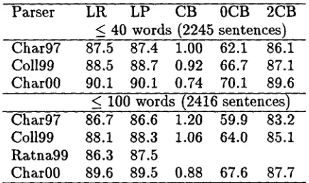
Parser LR LP CB 0CB 2CB < 40 words (2245 sentences) Char97 87.5 87.4 1.00 62.1 86.1 Co1199 88.5 88.7 0.92 66.7 87.1 Char00 90.1 90.1 0.74 70.1 89.6 < 100 words (2416 sentences) Char97 86.7 86.6 1.20 59.9 83.2 Coll99 88.1 88.3 1.06 64.0 85.1 Ratna99 86.3 87.5

Char00 89.6 89.5 0.88 67.6 87.7

Figure 1: Parsing results c o m p a r e d with previous work

five s m o o t h e d probability distributions, one each for L~, M,

Ri, t,

and h. T h e equation for the (unsmoothed) conditional probability distribution for t is given in Equation 7. T h e other four equations can be found in a longer version of this paper available on the a u t h o r ' s website (www.cs.brown.edu/~.,ec). L and R are conditioned on three previous labels so we are using a third-order Markov g r a m m a r . Also, t h e label of the parent constituent Ip is conditioned upon even when it is not obviously related to the further conditioning events. This is due to t h e importance of this factor in parsing, as noted in,

e.g., [14].

In keeping with t h e s t a n d a r d m e t h o d o l o g y [5, 9,10,15,17], we used the Penn Wall Street Jour- nal tree-bank [16] with sections 2-21 for training, section 23 for testing, and section 24 for development (debugging and tuning).

P e r f o r m a n c e on the test corpus is measured using the s t a n d a r d measures from [5,9,10,17]. In particular, we measure labeled precision (LP) and recall (LR), average n u m b e r of cross- brackets per sentence (CB), percentage of sentences with zero cross brackets (0CB), and percentage of sentences with < 2 cross brackets (2CB). Again as s t a n d a r d , we take separate m e a s u r e m e n t s for all sentences of length <_ 40 and all sentences of length < 100. Note t h a t the definitions of labeled precision and recall are those given in [9] and used in all of t h e previous work. As noted in [5], these definitions typically give results a b o u t 0.4% higher t h a n t h e more obvious ones. T h e results for t h e new parser as well as for the previous top-three individual parsers on this corpus are given in Figure 1.

As is typical, all of the s t a n d a r d measures tell p r e t t y much t h e same story, with the new parser outperforming the other three parsers. Looking in particular at t h e precision and recall figures, t h e new parser's give us a 13% error reduction over the best of the previous work, Co1199 [9].

5 Discussion

In the previous sections we have concentrated

on the relation of the parser to a m a x i m u m - entropy approach, the aspect of t h e parser t h a t is most novel. However, we do not think this aspect is the sole or even t h e most i m p o r t a n t reason for its comparative success. Here we list w h a t we believe to be the most significant con- tributions and give some experimental results on how well the program behaves w i t h o u t them. We take as our s t a r t i n g point t h e parser labled Char97 in Figure 1 [5], as t h a t is t h e p r o g r a m from which our c u r r e n t parser derives. T h a t parser, as s t a t e d in Figure 1, achieves an average precision/recall of 87.5. As noted in [5], t h a t s y s t e m is based upon a "tree-bank grammar" - - a g r a m m a r read directly off the training corpus. This is as opposed to t h e "Markov- g r a m m a r " approach used in t h e c u r r e n t parser. Also, the earlier parser uses two techniques not employed in t h e c u r r e n t parser. First, it uses a clustering scheme on words to give t h e sys- t e m a "soft" clustering of heads and sub-heads. (It is "soft" clustering in t h a t a word can be- long to more t h a n one cluster with different weights - - the weights express the probability of producing the word given t h a t one is going to produce a word from t h a t cluster.) Second, Char97 uses unsupervised learning in t h a t the original system was run on a b o u t t h i r t y million words of unparsed text, t h e o u t p u t was taken as "correct", and statistics were collected on t h e resulting parses. W i t h o u t these enhance- ments Char97 performs at the 86.6% level for sentences of length < 40.

In this section we evaluate t h e effects of the various changes we have m a d e by running various versions of our current program. To avoid repeated evaluations based upon t h e testing corpus, here our evaluation is based upon sentences of length < 40 from the development corpus. We note here t h a t this corpus is s o m e w h a t more difficult t h a n t h e "official" test corpus. For example, t h e final version of our system

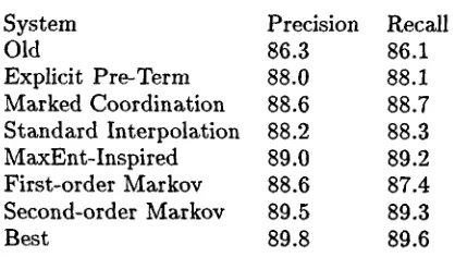
[image:5.612.109.326.100.229.2]

(6)

System Precision Recall

Old 86.3 86.1

Explicit Pre-Term 88.0 88.1 Marked Coordination 88.6 88.7 Standard Interpolation 88.2 88.3 MaxEnt-Inspired 89.0 89.2 First-order Markov 88.6 87.4 Second-order Markov 89.5 89.3

Best 89.8 89.6

Figure 2: Labeled precision/recall for length < 40, development corpus

achieves an average precision/recall of 90.1% on the test corpus but an average precision/recall of only 89.7% on the development corpus. This is indicated in Figure 2, where the model labeled "Best" has precision of 89.8% and recall of 89.6% for an average of 89.7%, 0.4% lower than the results on the official test corpus. This is in accord with our experience that development- corpus results are from 0.3% to 0.5% lower than those obtained on the test corpus.

The model labeled "Old" attempts to recreate the Char97 system using the current program. It makes no use of special maximum-entropy- inspired features (though their presence made it much easier to perform these experiments), it does not guess the pre-terminal before guessing the lexical head, and it uses a tree-bank g r a m m a r rather than a Markov grammar. This parser achieves an average precision/recall of 86.2%. This is consistent with the average precision/recall of 86.6% for [5] mentioned above, as the latter was on the test corpus and the for- mer on the development corpus.

Between the Old model and the Best model, Figure 2 gives precision/recall measurements for several different versions of our parser. One of the first and without doubt the most significant change we made in the current parser is to move from two stages of probabilistic decisions at each node to three. As already noted, Char97 first guesses the lexical head of a constituent and then, given the head, guesses the

PCFG

rule used to expand the constituent in question. In contrast, the current parser first guesses the head's pre~terminal, then the head, and then the expansion. It turns out that usefulness of this process had a/ready been discovered by Collins

[10], who in turn notes (personal communica- tion) that it was previously used by Eisner [12]. However, Collins in [10] does not stress the decision to guess the head's pre-terminal first, and it might be lost on the casual reader. Indeed, it was lost on the present author until he went back after the fact and found it there. In Figure 2 we show that this one factor improves performance by nearly 2%.

It may not be obvious why this should make so great a difference, since most words are ef- fectively unambiguous. (For example, part-of- speech tagging using the most probable pre- terminal for each word is 90% accurate [8].) We believe that two factors contribute to this performance gain. The first is simply that if we first guess the pre~terminal, when we go to guess the head the first thing we can condition upon is the pre-terminal, i.e., we compute

p(h I

t). This quantity is a relatively intuitive one (as, for example, it is the quantity used in a

PCFG

to re- late words to their pre-terminals) and it seems particularly good to condition upon here since we use it, in effect, as the unsmoothed probability upon which all smoothing of

p(h)

is based. This one '~fix" makes slightly over a percent difference in the results.

The second major reason why first guessing the pre-terminal makes so much difference is that it can be used when backing off the lexical head in computing the probability of the rule expansion. For example, when we first guess the lexical head we can move from computing

p(r I 1, lp, h)

to

p(r I l,t, lp, h).

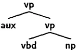
So, e.g., even if the word "conflating" does not appear in the training corpus (and it does not)~ the "ng" end- ing allows our program to guess with relative security that the word has the vbg pre-terminal, and thus the probability of various rule expansions can be considerable sharpened. For example, the tree-bank PCFG probability of the rule "vp --+ vbg np" is 0.0145, whereas once we condition on the fact that the lexical head is a vbg we get a probability of 0.214. [image:6.612.90.299.86.204.2]

(7)

vp

aux vp

vbd np

Figure 3: Verb phrase with both main and auxiliary verbs

parent will itself be an np, and similarly for a vp. But nps and vps can occur with np and vp parents in non-coordinate structures as well. For example, in the Penn Treebank a vp with both main and auxiliary verbs has the structure shown in Figure 3. Note t h a t the subordinate vp has a vp parent.

T h u s np and vp parents of constituents are marked to indicate if the parents are a coordinate structure. A vp coordinate structure is defined here as a constituent with two or more vp children, one or more of the constituents comma, cc, conjp (conjunctive phrase), and nothing else; coordinate np phrases are defined similarly. Something very much like this is done in [15]. As shown in Figure 2, conditioning on this information gives a 0.6% improvement. We believe t h a t this is mostly due to improvements in guessing the sub-constituent's pre-terminai and head. Given we are already at the 88% level of accuracy, we judge a 0.6% improvement to be very much worth while.

Next we add the less obvious conditioning events noted in our previous discussion of the final model - - grandparent label I a and left sibling label

lb.

W h e n we do so using our maximum-entropy-inspired conditioning, we get another 0.45% improvement in average precision/recall, as indicated in Figure 2 on the line labeled "MaocEnt-Inspired'. Note t h a t we also tried including this information using a standard deleted-interpolation model. The results here are shown in the line "Standard Interpola- tion". Including this information within a standard deleted-interpolation model causes a 0.6% decrease from the results using the less conventional model. Indeed, the resulting performance is worse t h a n not using this information at all.

Up to this point all the models considered in this section are tree-bank g r a m m a r models. T h a t is, the P C F G g r a m m a r rules are read directly off the training corpus. As already noted,

our best model uses a Markov-grammar approach. As one can see in Figure 2, a first- order Markov g r a m m a r (with all the aforemen- tioned improvements) performs slightly worse than the equivalent tree-bank-grammar parser. However, a second-order g r a m m a r does slightly better and a third-order g r a m m a r does significantly better than the tree-bank parser.

6 C o n c l u s i o n

We have presented a lexicalized Markov gram- m a r parsing model t h a t achieves (using the now standard t r a i n i n g / t e s t i n g / d e v e l o p m e n t sections of the Penn treebank) an average precision/recall of 91.1% on sentences of length < 40 and 89.5% on sentences of length < 100. This corresponds to an error reduction of 13% over the best previously published single parser results on this test set, those of Collins [9]. T h a t the previous three best parsers on this test [5,9,17] all perform within a percentage point of each other, despite quite different ba- sic mechanisms, led some researchers to won- der if there might be some m a x i m u m level of parsing performance t h a t could be obtained using the treebank for training, and to conjecture t h a t perhaps we were at it. The results reported here disprove this conjecture. The results of [13] achieved by combining the afore- mentioned three-best parsers also suggest t h a t the limit on tree-bank trained parsers is much higher than previously thought. Indeed, it may be t h a t adding this new parser to the mix may yield still higher results.

From our perspective, perhaps the two most i m p o r t a n t numbers to come out of this research are the overall error reduction of 13% over the results in [9] and the intermediate- result improvement of nearly 2% on labeled precision/recall due to the simple idea of guessing the bead's pre-terminal before guessing the head. Neither of these results were anticipated at the start of this research.

As noted above, the main methodological innovation presented here is our "maximum- entropy-inspired" model for conditioning and smoothing. Two aspects of this model deserve some comment. The first is the slight, but important, improvement achieved by using this model over conventional deleted interpolation, as indicated in Figure 2. We expect t h a t as

[image:7.612.171.251.90.142.2]

(8)

we experiment with other, more semantic conditioning information, the importance of this aspect of the model will increase.

More important in our eyes, though, is the flexibility of the maximum-entropy-inspired model. Though in some respects not quite as flexible as true maximum entropy, it is much simpler and, in our estimation, has benefits when it comes to smoothing. Ultimately it is this flexibility that let us try the various conditioning events, to move on to a Markov grammar approach, and to try several Markov grammars of different orders, without significant pro- gramming. Indeed, we initiated this line of work in an attempt to create a parser that would be flexible enough to allow modifications for parsing down to more semantic levels of detail. It is to this project that our future parsing work will be devoted.

R e f e r e n c e s

1. BERGER, A. L., PIETRA, S. A. D. AND PIETRA, V. J. D. A maximum entropy approach to natural language processing. Com- putational Linguistics 22 1 (1996), 39-71. 2. CARABALLO, S. AND CHARNIAK, E. New

figures of merit for best-first probabilistic chart parsing. Computational Linguistics 24 (1998), 275-298.

3. CHARNIAK, E. Tree-bank grammars. In Proceedings of the Thirteenth National Conference on Artificial Intelligence. AAAI Press/MIT Press, Menlo Park, 1996, 1031- 1036.

4. CHARNIAK, E. Expected-frequency interpolation. Department of Computer Science, Brown University, Technical Report CS96-37, 1996.

5.

CHARNIAK, E.

Statistical parsing with a context-free g r a m m a r and word statistics. In Proceedings of the Fourteenth National Conference on Artificial Intelligence. AAAI Press/MIT Press, Menlo Park, CA, 1997, 598-603.

6. CHARNIAK, E. Statistical techniques for natural language parsing. A I Magazine 18 4 (1997), 33-43.

7. CHARNIAK, E., GOLDWATER, S. AND JOHN- SON, M. Edge-based best-first chart pars- ing. In Proceedings of the Sixth Workshop on Very Large Corpora. 1998, 127-133. 8. CHARNIAK, E., HENDRICKSON, C., JACOB-

SON, N. AND PERKOWITZ, M. Equations for part-of-speech tagging. In Proceedings of the Eleventh National Conference on Arti- ficial Intelligence. AAAI Press/MIT Press, Menlo Park, 1993, 784-789.

9. COLLINS, M. Head-Driven Statistical Mod- els for Natural Language Parsing. University of Pennsylvania, Ph.D. Disseration, 1999. 10. COLLINS, M. J. Three generative lexicalised

models for statistical parsing. In Proceedings of the 35th Annual Meeting of the ACL. 1997, 16-23.

11. DARROCH, J. N. AND RATCLIFF, D. Gener- alized iterative scaling for log-linear models. Annals of Mathematical Statistics 33 (1972), 1470-1480.

12. EISNER~ J. M. An empirical comparison of probability models for dependency grammar. Institute for Research in Cognitive Science, University of Pennsylvania, Technical Report IRCS-96-11, 1996.

13. HENDERSON, J. C. AND BRILL, E. Exploit- ing diversity in natural language process- ing: combining parsers. In 1999 Joint Sigdat Conference on Empirical Methods in Natu- red Language Processing and Very Large Cor- pora. ACL, New Brunswick N J, 1999, 187-

194.

14. JOHNSON, M. PCFG models of linguistic tree representations. Computational Linguis- tics 24 4 (1998), 613-632.

15. MAGERMAN, D . M . Statistical decision-tree models for parsing. In Proceedings of the 33rd Annual Meeting of the Association for Com- putational Linguistics. 1995, 276-283.

16. MARCUS, M. P., SANTORINI, B. AND MARCINKIEWICZ, M. A. Building a large annotated corpus of English: the Penn tree- bank. Computational Linguistics 19 (1993), 313-330.