Modelling Annotator Bias with Multi-task Gaussian Processes:
An Application to Machine Translation Quality Estimation
Trevor Cohn and Lucia Specia Department of Computer Science
University of Sheffield Sheffield, United Kingdom
{t.cohn,l.specia}@sheffield.ac.uk
Abstract
Annotating linguistic data is often a com-plex, time consuming and expensive en-deavour. Even with strict annotation guidelines, human subjects often deviate in their analyses, each bringing different biases, interpretations of the task and lev-els of consistency. We present novel tech-niques for learning from the outputs of multiple annotators while accounting for annotator specific behaviour. These tech-niques use multi-task Gaussian Processes to learn jointly a series of annotator and metadata specific models, while explicitly representing correlations between models which can be learned directly from data. Our experiments on two machine trans-lation quality estimation datasets show uniform significant accuracy gains from multi-task learning, and consistently out-perform strong baselines.
1 Introduction
Most empirical work in Natural Language Pro-cessing (NLP) is based on supervised machine learning techniques which rely on human anno-tated data of some form or another. The annota-tion process is often time consuming, expensive, and prone to errors; moreover there is often con-siderable disagreement amongst annotators.
In general, the predominant perspective to deal with these data annotation issues in previous work has been that there is a single underlyingground truth, and that the annotations collected are noisy and/or biased samples of this. The challenge is then one of quality control, in order to process the data by filtering, averaging or similar to dis-til the truth. We posit that this perspective is too limiting, especially with respect to linguis-tic data, where each individual’s idiolect and lin-guistic background can give rise to many different
– and yet equally valid – truths. Particularly in highly subjective annotation tasks, the differences between annotators cannot be captured by simple models such as scaling all instances of a certain annotator by a factor. They can originate from a number of nuanced aspects. This is the case, for example, of annotations on the quality of sen-tences generated using machine translation (MT) systems, which are often used to buildquality es-timationmodels (Blatz et al., 2004; Specia et al., 2009) – our application of interest.
In addition to annotators’ own perceptions and expectations with respect to translation quality, a number of factors can affect their judgements on specific sentences. For example, certain anno-tators may prefer translations produced by rule-based systems as these tend to be more grammati-cal, while others would prefer sentences produced by statistical systems with more adequate lexical choices. Likewise, some annotators can be biased by the complexity of the source sentence: lengthy sentences are often (subconsciously) assumed to be of low quality by some annotators. An ex-treme case is the judgement of quality through post-editingtime: annotators have different typing speeds, as well as levels of expertise in the task of post-editing, proficiency levels in the language pair, and knowledge of the terminology used in particular sentences. These variations result in time measurements that are not comparable across annotators. Thus far, the use of post-editing time has been done on an per-annotator basis (Specia, 2011), or simply averaged across multiple transla-tors (Plitt and Masselot, 2010), both strategies far from ideal.
Overall, these myriad of factors affecting qual-ity judgements make the modelling of multiple annotators a very challenging problem. This problem is exacerbated when annotations are provided by non-professional annotators, e.g., through crowdsourcing – a common strategy used
to make annotation cheaper and faster, however at the cost of less reliable outcomes.
Most related work on quality assurance for data annotation has been developed in the context of crowdsourcing. Common practices include fil-tering out annotators who substantially deviate from a gold-standard set or present unexpected behaviours (Raykar et al., 2010; Raykar and Yu, 2012), or who disagree with others using, e.g., ma-jority or consensus labelling (Snow et al., 2008; Sheng et al., 2008). Another relevant strand of work aims to model legitimate, systematic biases in annotators (including both non-experts and ex-perts), such as the fact that some annotators tend to be more negative than others, and that some annotators use a wider or narrower range of val-ues (Flach et al., 2010; Ipeirotis et al., 2010). However, with a few exceptions in Computer Vi-sion (e.g., Whitehill et al. (2009), Welinder et al. (2010)), existing work disregard metadata and its impact on labelling.
In this paper we model the task of predicting the quality of sentence translations using datasets that have been annotated by several judges with differ-ent levels of expertise and reliability, containing translations from a variety of MT systems and on a range of different types of sentences. We ad-dress this problem using multi-task learning in which we learn individual models for each context (the task, incorporating the annotator and other metadata: translation system and the source sen-tence) while also modelling correlations between tasks such that related tasks can mutually inform one another. Our use of multi-task learning allows the modelling of a diversity of truths, while also recognising that they are rarely independent of one another (annotators often agree) by explicitly ac-counting for inter-annotator correlations.
Our approach is based on Gaussian Processes (GPs) (Rasmussen and Williams, 2006), a ker-nelised Bayesian non-parametric learning frame-work. We develop multi-task learning models by representing intra-task transfer simply and explic-itly as part of a parameterised kernel function. GPs are an extremely flexible probabilistic framework and have been successfully adapted for multi-task learning in a number of ways, e.g., by learning multi-task correlations (Bonilla et al., 2008), mod-elling task variance (Groot et al., 2011) or per-annotator biases (Rogers et al., 2010). Our method builds on the work of Bonilla et al. (2008) by
explicitly modelling intra-task transfer, which is learned automatically from the data, in order to ro-bustly handle outlier tasks and task variances. We show in our experiments on two translation qual-ity datasets that these multi-task learning strate-gies are far superior to training individual per-task models or a single pooled model, and moreover that our multi-task learning approach can achieve similar performance to these baselines using only a fraction of the training data.
In addition to showing empirical performance gains on quality estimation applications, an im-portant contribution of this paper is in introduc-ing Gaussian Processes to the NLP community,1
a technique that has great potential to further per-formance in a wider range of NLP applications. Moreover, the algorithms proposed herein can be adapted to improve future annotation efforts, and subsequent use of noisy crowd-sourced data.
2 Quality Estimation
Quality estimation (QE) for MT aims at providing an estimate on the quality of each translated seg-ment – typically a sentence – without access to ref-erence translations. Work in this area has become increasingly popular in recent years as a conse-quence of the widespread use of MT among real-world users such as professional translators. Ex-amples of applications of QE include improving post-editing efficiency by filtering out low qual-ity segments which would require more effort and time to correct than translating from scratch (Spe-cia et al., 2009), selecting high quality segments to be published as they are, without post-editing (Soricut and Echihabi, 2010), selecting a trans-lation from either an MT system or a transtrans-lation memory for post-editing (He et al., 2010), select-ing the best translation from multiple MT sys-tems (Specia et al., 2010), and highlighting sub-segments that need revision (Bach et al., 2011).
QE is generally addressed as a machine learn-ing task uslearn-ing a variety of linear and kernel-based regression or classification algorithms to induce models from examples of translations described through a number of features and annotated for quality. For an overview of various algorithms and features we refer the reader to the WMT12 shared task on QE (Callison-Burch et al., 2012).
While initial work used annotations derived
1We are not strictly the first, Polajnar et al. (2011) used
from automatic MT evaluation metrics (Blatz et al., 2004) such as BLEU (Papineni et al., 2002) at training time, it soon became clear that human labels result in significantly better models (Quirk, 2004). Current work at sentence level is thus based on some form of human supervision.
As typical of subjective annotation tasks, QE datasets should contain multiple annotators to lead to models that are representative. Therefore, work in QE faces all common issues regarding variabil-ity in annotators’ judgements. The following are a few other features that make our datasets particu-larly interesting:
• In order to minimise annotation costs, trans-lation instances are often spread among anno-tators, such that each instance is only labelled by one or a few judges. In fact, for a sizeable dataset (thousands of instances), the annota-tion of a complete dataset by a single judge may become infeasible.
• It is often desirable to include alternative translations of source sentences produced by multiple MT systems, which requires multi-ple annotators for unbiased judgements, par-ticularly for labels such as post-editing time (a translation seen a second time will require less editing effort).
• For crowd-sourced annotations it is often im-possible to ensure that the same annotators will label the same subset of cases.
These features – which are also typical of many other linguistic annotation tasks – make the learn-ing process extremely challenglearn-ing. Learnlearn-ing mod-els from datasets annotated by multiple annotators remains an open challenge in QE, as we show in Section 4. In what follows, we present our QE datasets in more detail.
2.1 Datasets
We use two freely available QE datasets to experi-ment with the techniques proposed in this paper:2
WMT12: This dataset was distributed as part of the WMT12 shared task on QE (Callison-Burch et al., 2012). It contains 1,832instances for
train-ing, and 422 for test. The English source
sen-tences are a subset of WMT09-12 test sets. The Spanish MT outputs were created using a standard PBSMT Moses engine. Each instance was anno-tated with post-editing effort scores from highest
2Both datasets can be downloaded fromhttp://www.
dcs.shef.ac.uk/˜lucia/resources.html.
effort (score 1) to lowest effort (score 5), where each score identifies an estimated percentage of the MT output that needs to be corrected. The post-editing effort scores were produced indepen-dently by three professional translators based on a previously post-edited translation by a fourth translator. In an attempt to accommodate for sys-tematic biases among annotators, the final effort score was computed as the weighted average be-tween the three PE-effort scores, with more weight given to the judges with higher standard deviation from their own mean score. This resulted in scores spread more evenly in the[1,5]range.
WPTP12: This dataset was distributed by Ko-ponen et al. (2012). It contains299English
sen-tences translated into Spanish using two or more of eight MT systems randomly selected from all system submissions for WMT11 (Callison-Burch et al., 2011). These MT systems range from on-line and customised SMT systems to commercial rule-based systems. Translations were post-edited by humans while time was recorded. The labels are the number of seconds spent by a translator editing a sentence normalised by source sentence length. The post-editing was done by eight na-tive speakers of Spanish, including five profes-sional translators and three translation students. Only20 translations were edited by all eight an-notators, with the remaining translations randomly distributed amongst them. The resulting dataset contains 1,624 instances, which were randomly
split into1,300for training and300for test.
Ac-cording to the analysis in (Koponen et al., 2012), while on average certain translators were found to be faster than others, their speed in post-editing individual sentences varies considerably, i.e., cer-tain translators are faster at cercer-tain sentences. To our knowledge, no previous work has managed to successfully model the prediction of post-editing time from datasets with multiple annotators.
3 Gaussian Process Regression
func-tions. In this paper we consider Gaussian Pro-cesses (GP) (Rasmussen and Williams, 2006), a probabilistic machine learning framework incor-porating kernels and Bayesian non-parametrics, widely considered state-of-the-art for regression. Despite this GPs have not been used widely to date in statistical NLP. GPs are particularly suitable for modelling QE for a number of reasons: 1) they explicitly model uncertainty, which is rife in QE datasets; 2) they allow fitting of expressive kernels to data, in order to modulate the effect of features of varying usefulness; and 3) they can naturally be extended to model correlated tasks using multi-task kernels. We now give a brief overview of GPs, following Rasmussen and Williams (2006).
In our regression task3 the data consists of n
pairs D = {(xi, yi)}, where xi ∈ RF is a F
-dimensional feature vector and yi ∈ Ris the
re-sponse variable. Each instance is a translation and the feature vector encodes its linguistic features; the response variable is a numerical quality judge-ment: post editing time or likert score. As usual, the modelling challenge is to automatically predict the value ofybased on thexfor unseen test input. GP regression assumes the presence of a la-tent function, f : RF → R, which maps from
the input space of feature vectors x to a scalar. Each response value is then generated from the function evaluated at the corresponding data point, yi = f(xi) +η, where η ∼ N(0, σ2n) is added
white-noise. Formallyfis drawn from a GP prior,
f(x)∼ GP 0, k(x,x0) ,
which is parameterised by a mean (here, 0) and a covariance kernel function k(x,x0). The
ker-nel function represents the covariance (i.e., sim-ilarities in the response) between pairs of data points. Intuitively, points that are in close proxim-ity should have high covariance compared to those that are further apart, which constrains f to be a smoothly varying function of its inputs. This intu-ition is embodied in the squared exponential ker-nel (a.k.a.radial basis function or Gaussian),
k(x,x0) =σ2fexp
−12(x−x0)TA−1(x−x0)
(1) whereσ2f is a scaling factor describing the overall levels of variance, andA= diag(a)is a diagonal 3Our approach generalises to classification, ranking
(ordi-nal regression) or various other training objectives, including mixtures of objectives. In this paper we use regression for simplicity of exposition and implementation.
matrix of length scales, encoding the smoothness of functionsf with respect to each feature. Non-uniform length scales allow for different degrees of smoothness off in each dimension, such that e.g., for unimportant features f is relatively flat whereas for very important features f is jagged, such that a small change in the feature value has a large effect. When the values of aare learned automatically from data, as we do herein, this is referred to as theautomatic relevance determina-tion(ARD) kernel.
Given the generative process defined above, we formulate prediction as Bayesian inference under the posterior, namely
p(y∗|x∗,D) =
Z
f
p(y∗|x∗, f)p(f|D)
where x∗ is a test input and y∗ is its response value. The posteriorp(f|D) reflects our updated
belief over possible functions after observing the training setD, i.e., f should pass close to the re-sponse values for each training instance (but need not fit exactly due to additive noise). This is bal-anced against the smoothness constraints that arise from the GP prior. The predictive posterior can be solved analytically, resulting in
y∗ ∼ N kT∗(K+σn2I)−1y, (2)
k(x∗,x∗)−kT∗(K+σn2I)−1k∗
wherek∗ = [k(x∗,x1) k(x∗,x2)· · ·k(x∗,xn)]T
are the kernel evaluations between the test point and the training set, and {Kij = k(xi,xj)} is
the kernel (gram) matrix over the training points. Note that the posterior in Eq. 2 includes not only the expected response (the mean) but also the vari-ance, encoding the model’s uncertainty, which is important for integration into subsequent process-ing, e.g., as part of a larger probabilistic model.
GP regression also permits an analytic for-mulation of the marginal likelihood, p(y|X) =
R
fp(y|X, f)p(f), which can be used for model
training (X are the training inputs). Specifically, we can derive the gradient of the (log) marginal likelihood with respect to the model hyperparam-eters (i.e.,a, σn, σsetc.) and thereby find the type
with the (good) solutions found for simpler mod-els, thereby avoiding poor local optima. We refer the reader to Rasmussen and Williams (2006) for further details.
At first glance GPs resemble SVMs, which also admit kernels such as the popular squared expo-nential kernel in Eq. 1. The key differences are that GPs are probabilistic models and support ex-act Bayesian inference in the case of regression (approximate inference is required for classifica-tion (Rasmussen and Williams, 2006)). Moreover GPs provide greater flexibility in fitting the ker-nel hyperparameters even for complex composite kernels. In typical usage, the kernel hyperparam-eters for an SVM are fit using held-out estima-tion, which is inefficient and often involves ty-ing together parameters to limit the search com-plexity (e.g., using a single scale parameter in the squared exponential). Multiple-kernel learning (G¨onen and Alpaydın, 2011) goes some way to ad-dressing this problem within the SVM framework, however this technique is limited to reweighting linear combinations of kernels and has high com-putational complexity.
3.1 Multi-task Gaussian Process Models
Until now we have considered a standard regres-sion scenario, where each training point is labelled with a single output variable. In order to model multiple different annotators jointly, i.e., multi-task learning, we need to extend the model to han-dle many tasks. Conceptually, we can consider the multi-task model drawing a latent function for each task,fm(x), wherem ∈1, ..., M is the task
identifier. This function is then used to explain the response values for all the instances for that task (subject to noise). Importantly, for multi-task learning to be of benefit, the prior over{fm}must
correlate the functions over different tasks, e.g., by imposing similarity constraints between the values forfm(x)andfm0(x).
We can consider two alternative perspectives for framing the multi-task learning problem: ei-therisotopicwhere we associate each input point x with a vector of outputs, y ∈ RM, one for
each of the M tasks; or heterotopicwhere some of the outputs are missing, i.e., tasks are not con-strained to share the same data points (Alvarez et al., 2011). Given the nature of our datasets, we opted for the heterotopic approach, which can han-dle both singly annotated and multiply annotated
data. This can be implemented by augmenting each input point with an additional task identity feature, which is paired with a singley response, and integrated into a GP model with the standard training and inference algorithms.4
In moving to a task-augmented data representa-tion, we need to revise our kernel function. We use a separable multi-task kernel (Bonilla et al., 2008; Alvarez et al., 2011) of the form
k (x, d),(x0, d0)=kdata(x,x0)Bd,d0, (3)
wherekdata(x,x0)is a standard kernel over the
in-put points, typically a squared exponential (see Eq. 1), andB ∈RD×D is a positive semi-definite matrix encoding task covariances. We develop a series of increasingly complex choices for B, which we compare empirically in Section 4.2:
Independent The simplest case is whereB=I, i.e., all pairs of different tasks have zero covari-ance. This corresponds to independent modelling of each task, although all models share the same data kernel, so this setting is not strictly equiva-lent to independent training with independent per-task data kernels (with different hyperparameters). Similarly, we might choose to use a single noise variance,σn2, or an independent noise variance hy-perparameter per task.
Pooled Another extreme is B = 1, which ig-nores the task identity, corresponding to pooling the multi-task data into one large set. Groot et al. (2011) present a method for applying GPs for modelling multi-annotator data using this pool-ingkernel with independent per-task noise terms. They show on synthetic data experiments that this approach works well at extracting the signal from noise-corrupted inputs.
Combined A simple approach for B is a weighted combination ofIndependentandPool, i.e.,B =1+aI, where the hyperparametera≥0
controls the amount of inter-task transfer between each task and the global ‘pooled’ task.5 For
dis-similar tasks, a high value ofaallows each task to be modelled independently, while for more simi-lar tasks low aallows the use of a large pool of
4Note that the separable kernel (Eq. 3) gives rise to block
structured kernel matrices which permit various optimisa-tions (Bonilla et al., 2008) to reduce the computational com-plexity of inference, e.g., the matrix inversion in Eq. 2.
5Note that larger values ofaneed not affect the overall
similar data. A scaled version of this kernel has been shown to correspond to mean regularisation in SVMs when combined with a linear data ker-nel (Evgeniou et al., 2006). A similar multi-task kernel was proposed by Daum´e III (2007), using a linear data kernel anda = 1, which has shown
to result in excellent performance across a range of NLP problems. In contrast to these earlier ap-proaches, we learn the hyperparameteradirectly, fitting the relative amounts of inter- versus intra-task transfer to the dataset.
Combined+ We consider an extension to the
Combined kernel, B = 1 + diag(a), ad ≥ 0
in which each task has a different hyperparameter modulating its independence from the global pool. This additional flexibility can be used, e.g., to al-low individual outlier annotators to be modelled independently of the others, by assigning a high value toad. In contrast, Combinedties together
the parameters for all tasks, i.e., all annotators are assumed to have similar quality in that they devi-ate from the mean to the same degree.
3.2 Integrating metadata
The approaches above assume that the data is split into an unstructured set ofM tasks, e.g., by anno-tator. However, it is often the case that we have additional information about each data instance in the form of metadata. In our quality estimation experiments we consider as metadata the MT sys-tem which produced the translation, and the iden-tity of the source sentence being translated. Many other types of metadata, such as the level of expe-rience of the annotator, could also be used. One way of integrating such metadata would be to de-fine a separate task for every observed combina-tion of metadata values, in which case we treat the metadata as a task descriptor. Doing so naively would however incur a significant penalty, as each task will have very few training instances result-ing in inaccurate models, even with the inter-task kernel approaches defined above.
We instead extend the task-level kernels to use the task descriptors directly to represent task cor-relations. LetB(i) be a square covariance matrix for theithtask descriptor ofM, with a column and
row for each value (e.g., annotator identity, trans-lation system, etc.). We redefine the task level ker-nel using paired inputs (x,m), wherem are the
task descriptors,
k (x,m),(x0,m0)=kdata(x,x0)
M
Y
i=1
B(mi)
i,m0i.
This is equivalent to using a structured task-kernel B = B(1)⊗B(3) ⊗ · · · ⊗B(M) where⊗is the
Kronecker product. Using this formulation we can consider any of the above choices for B applied to each task descriptor. In our experiments we consider theCombinedandCombined+kernels, which allow the model to learn the relative impor-tance of each descriptor in terms of independent modelling versus pooling the data.
4 Multi-task Quality Estimation
4.1 Experimental Setup
Feature sets: In all experiments we use17
shal-low QE features that have been shown to perform well in previous work. These were used by a highly competitive baseline entry in the WMT12 shared task, and were extracted here using the sys-tem provided by that shared task.6 They include
simple counts, e.g., the tokens in sentences, as well as source and target language model proba-bilities. Each feature was scaled to have zero mean and unit standard deviation on the training set.
Baselines: The baselines use the SVM regres-sion algorithm with radial basis function kernel and parametersγ,andCoptimised through grid-search and 5-fold cross validation on the training set. This is generally a very strong baseline: in the WMT12 QE shared task, only five out of 19 submissions were able to significantly outperform it, and only by including many complex additional features, tree kernels, etc. We also present µ, a trivial baseline based on predicting for each test instance the training mean (overall, and for spe-cific tasks).
GP: All GP models were implemented using the GPMLMatlab toolbox.7 Hyperparameter
optimi-sation was performed using conjugate gradient as-cent of the log marginal likelihood function, with up to 100 iterations. The simpler models were ini-tialised with all hyperparameters set to one, while more complex models were initialised using the
6The software used to extract these (and other)
fea-tures can be downloaded from http://www.quest. dcs.shef.ac.uk/
7http://www.gaussianprocess.org/gpml/
Model MAE RMSE
µ 0.8279 0.9899
SVM 0.6889 0.8201 Linear ARD 0.7063 0.8480 Squared exp. Isotropic 0.6813 0.8146 Squared exp. ARD 0.6680 0.8098
Rational quadratic ARD 0.6773 0.8238 Matern(5,2) 0.6772 0.8124 Neural network 0.6727 0.8103 Table 1: Single-task learning results on the
WMT12 dataset, trained and evaluated against the weighted averaged response variable. µ is a
baseline which predicts the training mean, SVM uses the same system as the WMT12 QE task, and the remainder are GP regression models with dif-ferent kernels (all include additive noise).
solution for a simpler model. For instance, mod-els using ARD kernmod-els were initialised from an equivalent isotropic kernel (which ties all the hy-perparameters together), and independent per-task noise models were initialised from a single noise model. This approach was more reliable than ran-dom restarts in terms of accuracy and runtime ef-ficiency.
Evaluation: We evaluate predictive accuracy using two measures: mean absolute error,
MAE = N1 PNi=1|yi−yˆi| and root mean square
error, RMSE =
q
1
N
PN
i=1(yi−yˆi)
2, where y
i
are the gold standard response values and yˆi are
the model predictions.
4.2 Results
Our experiments aim to demonstrate the efficacy of GP regression, both the single task and multi-task settings, compared to competitive baselines.
WMT12: Single task We start by comparing GP regression with alternative approaches using the WMT12dataset on the standard task of pre-dicting a weighted mean quality rating (as it was done in the WMT12 QE shared task). Table 1 shows the results for baseline approaches and the GP models, using a variety of different kernels (see Rasmussen and Williams (2006) for details of the kernel functions). From this we can see that all models do much better than the mean baseline and that most of the GP models have lower error than the state-of-the-art SVM. In terms of kernels, the linear kernel performs comparatively worse than non-linear kernels. Overall the squared
exponen-Model MAE RMSE
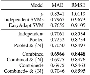
µ 0.8541 1.0119
Independent SVMs 0.7967 0.9673 EasyAdapt SVM 0.7655 0.9105 Independent 0.7061 0.8534 Pooled 0.7252 0.8754 Pooled &{N} 0.7050 0.8497 Combined 0.6966 0.8448
[image:7.595.338.496.62.193.2]Combined &{N} 0.6975 0.8476 Combined+ 0.6975 0.8463 Combined+ &{N} 0.7046 0.8595
Table 2: Results on the WMT12 dataset, trained and evaluated over all three annotator’s judge-ments. Shown above are the training mean base-lineµ, single-task learning approaches, and
multi-task learning models, with the columns showing macro average error rates over all three response values. All systems use a squared exponential ARD kernel in a product with the named task-kernel, and with added noise (per-task noise is de-noted{N}, otherwise has shared noise).
tial ARD kernel has the best performance under both measures of error, and for this reason we use this kernel in our subsequent experiments.
WMT12: Multi-task We now turn to the multi-task setting, where we seek to model each of the three annotators’ predictions. Table 2 presents the results. Note that here error rates are mea-sured over all of the three annotators’ judgements, and consequently are higher than those measured against their average response in Table 1. For com-parison, taking the predictions of the best model,
Combined, in Table 2 and evaluating its averaged prediction has a MAE of 0.6588 vs. the averaged gold standard, significantly outperforming the best model in Table 1.
There are a number of important findings in Ta-ble 2. First, the independently trained models do well, outperforming the pooled model with fixed noise, indicating that naively pooling the data is counter-productive and that there are annotator-specific biases. Including per-annotator noise to the pooled model provides a boost in performance, however the best results are obtained using the
[image:7.595.93.271.63.170.2]of independent noise is that differences between annotators can already be explained by the MTL model using the multi-task kernel, and need not be explained as noise.
The GP models significantly improve over the baselines, including an SVM trained inde-pendently and using the EasyAdapt method for multi-task learning (Daum´e III, 2007). While EasyAdapt showed an improvement over the in-dependent SVM, it was a long way short of the GP models. A possible explanation is that in EasyAdapt the multi-task sharing parameter is set at a = 1, which may not be appropriate for the task. In contrast theCombinedGP model learned a value ofa= 0.01, weighting the value of
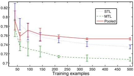
pool-ing much more highly than independent trainpool-ing. A remaining question is how these approaches cope with smaller datasets, where issues of data sparsity become more prevalent. To test this, we trained single-task, pooled and multi-task models on randomly sub-sampled training sets of differ-ent sizes, and plot their error rates in Figure 1. As expected, for very small datasets pooling out-performs single task learning, however for modest sized datasets of≥ 90 training instances pooling
was inferior. For all dataset sizes multi-task learn-ing is superior to the other approaches, maklearn-ing much better use of small and large training sets. The MTL model trained on 500 samples had an
MAE of0.7082±0.0042, close to the best results
from the full dataset in Table 2, despite using 1 9
as much data: here we use 1
3 as many training
instances where each is singly (cf. triply) anno-tated. The same experiments run with multiply-annotated instances showed much weaker perfor-mance, presumably due to the more limited sam-ple of input points and poorer fit of the ARD ker-nel hyperparameters. This finding suggests that our multi-task learning approach could be used to streamline annotation efforts by reducing the need for extensive multiple annotations.
WPTP12 This dataset involves predicting the post-editing time for eight annotators, where we seek to test our model’s capability to use addi-tional metadata. We model the logarithm of the per-word post-editing time, in order to make the response variable more comparable between an-notators and across sentences, and generally more Gaussian in shape. In Table 3 immediately we can see that the baseline of predicting the train-ing mean is very difficult to beat, and the trained
50 100 150 200 250 300 350 400 450 500
0.7 0.72 0.74 0.76 0.78 0.8 0.82
Training examples
[image:8.595.307.524.61.185.2]STL MTL Pooled
Figure 1: Learning curve comparing MAE for dif-ferent training methods on the WMT12 dataset, all using a squared exponential ARD data kernel and tied noise parameter. The MTL model uses the
Combinedtask kernel. Each point is the average
of 5 runs, and the error bars show±1s.d.
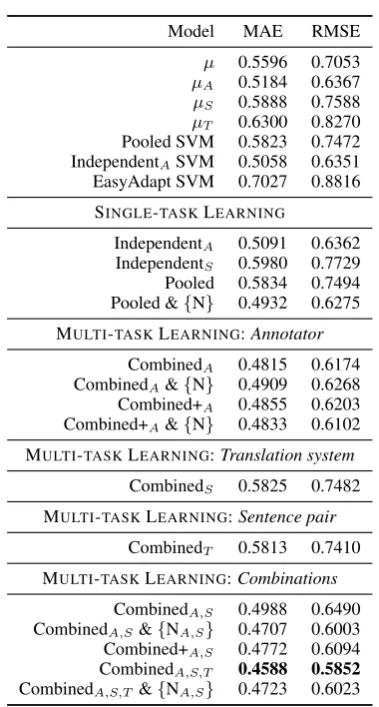
systems often do worse. Partitioning the data by annotator (µA) gives the best baseline result,
while there is less information from the MT sys-tem or sentence identity. Single-task learning per-forms only a little better than these baselines, al-though some approaches such as the naive pool-ing perform terribly. This suggests that the tasks are highly different to one another. Interestingly, adding the per-task noise models to the pooling ap-proach greatly improves its performance.
The multi-task learning methods performed best when using the annotator identity as the task de-scriptor, and less well for the MT system and sen-tence pair, where they only slightly improved over the baseline. However, making use of all these lay-ers of metadata together gives substantial further improvements, reaching the best result with Com-binedA,S,T. The effect of adding per-task noise to
these models was less marked than for the pooled models, as in the WMT12 experiments. Inspecting the learned hyperparameters, the combined mod-els learned a large bias towards independent learn-ing over poollearn-ing, in contrast to the WMT12 exper-iments. This may explain the poor performance of EasyAdapt on this dataset.
5 Conclusion
meta-Model MAE RMSE
µ 0.5596 0.7053 µA 0.5184 0.6367 µS 0.5888 0.7588 µT 0.6300 0.8270 Pooled SVM 0.5823 0.7472 IndependentASVM 0.5058 0.6351 EasyAdapt SVM 0.7027 0.8816 SINGLE-TASKLEARNING
IndependentA 0.5091 0.6362 IndependentS 0.5980 0.7729 Pooled 0.5834 0.7494 Pooled &{N} 0.4932 0.6275 MULTI-TASKLEARNING:Annotator
CombinedA 0.4815 0.6174 CombinedA&{N} 0.4909 0.6268 Combined+A 0.4855 0.6203 Combined+A&{N} 0.4833 0.6102 MULTI-TASKLEARNING:Translation system
CombinedS 0.5825 0.7482 MULTI-TASKLEARNING:Sentence pair
CombinedT 0.5813 0.7410 MULTI-TASKLEARNING:Combinations
[image:9.595.86.276.180.534.2]CombinedA,S 0.4988 0.6490 CombinedA,S&{NA,S} 0.4707 0.6003 Combined+A,S 0.4772 0.6094 CombinedA,S,T 0.4588 0.5852 CombinedA,S,T &{NA,S} 0.4723 0.6023 Table 3: Results on the WPTP12 dataset, using the log of the post-editing time per word as the response variable. Shown above are the training mean and SVM baselines, single-task learning and multi-task learning results (micro average). The subscripts denote the task split: annotator (A), MT system (S) and sentence identity (T).
data. Our experiments showed how our approach outperformed competitive baselines on two ma-chine translation quality regression problems, in-cluding the highly challenging problem of predict-ing post-editpredict-ing time.
In future work we plan to apply these techniques to new datasets, particularly noisy crowd-sourced data with much large numbers of annotators, as well as a wider range of task types and mixtures thereof (regression, ordinal regression, ranking, classification). We also have preliminary positive results for more advanced multi-task kernels, e.g., general dense matrices, which can induce clusters of related tasks.
Our multi-task learning approach has much wider application. Models of individual annota-tors could be used to train machine translation systems to optimise an annotator-specific quality measure, or in active learning for corpus annota-tion, where the model can suggest the most ap-propriate instances for each annotator or the best annotator for a given instance. Further, our ap-proach contributes to work based on cheap and fast crowdsourcing of linguistic annotation by min-imising the need for careful data curation and quality control.
Acknowledgements
This work was funded by PASCAL2 Harvest Pro-gramme, as part of the QuEst project: http: //www.quest.dcs.shef.ac.uk/. The au-thors would like to thank Neil Lawerence and James Hensman for advice on Gaussian Processes, the QuEst participants, particularly Jos´e Guil-herme Camargo de Souza and Eva Hassler, and the three anonymous reviewers.
References
Mauricio A. Alvarez, Lorenzo Rosasco, and Neil D. Lawrence. 2011. Kernels for vector-valued
func-tions: A review. Foundations and Trends in Machine
Learning, 4(3):195–266.
Nguyen Bach, Fei Huang, and Yaser Al-Onaizan. 2011. Goodness: a method for measuring machine
translation confidence. In the 49th Annual
Meet-ing of the Association for Computational LMeet-inguis- Linguis-tics: Human Language Technologies, pages 211– 219, Portland, Oregon.
Sanchis, and Nicola Ueffing. 2004. Confidence
Es-timation for Machine Translation. Inthe 20th
Inter-national Conference on Computational Linguistics (Coling 2004), pages 315–321, Geneva.
Edwin Bonilla, Kian Ming Chai, and Christopher Williams. 2008. Multi-task gaussian process
pre-diction. InAdvances in Neural Information
Process-ing Systems (NIPS).
Chris Callison-Burch, Philipp Koehn, Christof Monz, and Omar Zaidan. 2011. Findings of the 2011
work-shop on statistical machine translation. Inthe Sixth
Workshop on Statistical Machine Translation, pages 22–64, Edinburgh, Scotland.
Chris Callison-Burch, Philipp Koehn, Christof Monz, Matt Post, Radu Soricut, and Lucia Specia. 2012. Findings of the 2012 workshop on statistical
ma-chine translation. In the Seventh Workshop
on Statistical Machine Translation, pages 10–51, Montr´eal, Canada.
Hal Daum´e III. 2007. Frustratingly easy domain
adap-tation. In the 45th Annual Meeting of the
Associ-ation for ComputAssoci-ational Linguistics, Prague, Czech Republic.
Theodoros Evgeniou, Charles A. Micchelli, and Massi-miliano Pontil. 2006. Learning multiple tasks with
kernel methods. Journal of Machine Learning
Re-search, 6(1):615.
Peter A. Flach, Sebastian Spiegler, Bruno Gol´enia, Si-mon Price, John Guiver, Ralf Herbrich, Thore Grae-pel, and Mohammed J. Zaki. 2010. Novel tools to streamline the conference review process:
experi-ences from SIGKDD’09. SIGKDD Explor. Newsl.,
11(2):63–67, May.
Mehmet G¨onen and Ethem Alpaydın. 2011.
Multi-ple kernel learning algorithms. Journal of Machine
Learning Research, 12:2211–2268.
Perry Groot, Adriana Birlutiu, and Tom Heskes. 2011. Learning from multiple annotators with gaussian
processes. InProceedings of the 21st international
conference on Artificial neural networks - Volume Part II, ICANN’11, pages 159–164, Espoo, Finland. Yifan He, Yanjun Ma, Josef van Genabith, and Andy Way. 2010. Bridging smt and tm with
transla-tion recommendatransla-tion. In the 48th Annual
Meet-ing of the Association for Computational LMeet-inguis-
Linguis-tics, pages 622–630, Uppsala, Sweden.
Panagiotis G. Ipeirotis, Foster Provost, and Jing Wang. 2010. Quality management on amazon mechanical
turk. In Proceedings of the ACM SIGKDD
Work-shop on Human Computation, HCOMP ’10, pages 64–67, Washington DC.
Maarit Koponen, Wilker Aziz, Luciana Ramos, and Lucia Specia. 2012. Post-editing time as a
mea-sure of cognitive effort. In Proceedings of the
AMTA 2012 Workshop on Post-editing Technology and Practice, WPTP 2012, San Diego, CA.
Kishore Papineni, Salim Roukos, Todd Ward, and Wei-Jing Zhu. 2002. Bleu: a method for automatic
evaluation of machine translation. In the 40th
An-nual Meeting of the Association for Computational Linguistics, pages 311–318, Philadelphia, Pennsyl-vania.
Mirko Plitt and Franc¸ois Masselot. 2010. A productiv-ity test of statistical machine translation post-editing
in a typical localisation context. Prague Bull. Math.
Linguistics, 93:7–16.
Tamara Polajnar, Simon Rogers, and Mark Girolami. 2011. Protein interaction detection in sentences via
gaussian processes; a preliminary evaluation. Int. J.
Data Min. Bioinformatics, 5(1):52–72, February.
Christopher B. Quirk. 2004. Training a sentence-level
machine translation confidence metric. In
Proceed-ings of the International Conference on Language Resources and Evaluation, volume 4 ofLREC 2004, pages 825–828, Lisbon, Portugal.
Carl E. Rasmussen and Christopher K.I. Williams.
2006. Gaussian processes for machine learning,
volume 1. MIT press Cambridge, MA.
Vikas C. Raykar and Shipeng Yu. 2012. Eliminating spammers and ranking annotators for crowdsourced
labeling tasks.J. Mach. Learn. Res., 13:491–518.
Vikas C. Raykar, Shipeng Yu, Linda H. Zhao, Ger-ardo Hermosillo Valadez, Charles Florin, Luca Bo-goni, and Linda Moy. 2010. Learning from crowds.
J. Mach. Learn. Res., 99:1297–1322.
Simon Rogers, Mark Girolami, and Tamara Polajnar. 2010. Semi-parametric analysis of multi-rater data.
Statistics and Computing, 20(3):317–334.
Victor S. Sheng, Foster Provost, and Panagiotis G. Ipeirotis. 2008. Get another label? Improving data quality and data mining using multiple, noisy
la-belers. InProceedings of the 14th ACM SIGKDD,
KDD’08, pages 614–622, Las Vegas, Nevada.
Rion Snow, Brendan O’Connor, Daniel Jurafsky, and Andrew Y. Ng. 2008. Cheap and fast—but is it good? Evaluating non-expert annotations for natural
language tasks. Inthe 2008 Conference on
Empiri-cal Methods in Natural Language Processing, pages 254–263, Honolulu, Hawaii.
Radu Soricut and Abdessamad Echihabi. 2010.
Trustrank: Inducing trust in automatic translations
via ranking. Inthe 49th Annual Meeting of the
Asso-ciation for Computational Linguistics: Human Lan-guage Technologies, pages 612–621, Uppsala, Swe-den, July.
Lucia Specia, Marco Turchi, Nicola Cancedda, Marc Dymetman, and Nello Cristianini. 2009. Estimat-ing the Sentence-Level Quality of Machine
Trans-lation Systems. In the 13th Annual Meeting of
Lucia Specia, Dhwaj Raj, and Marco Turchi. 2010. Machine translation evaluation versus quality
esti-mation. Machine Translation, pages 39–50.
Lucia Specia. 2011. Exploiting Objective Annotations
for Measuring Translation Post-editing Effort. Inthe
15th Annual Meeting of the European Association for Machine Translation (EAMT’2011), pages 73– 80, Leuven.
Peter Welinder, Steve Branson, Serge Belongie, and Pietro Perona. 2010. The Multidimensional
Wis-dom of Crowds. InAdvances in Neural Information
Processing Systems, volume 23, pages 2424–2432. Jacob Whitehill, Paul Ruvolo, Ting-fan Wu, Jacob
Bergsma, and Javier Movellan. 2009. Whose vote should count more: Optimal integration of labels
from labelers of unknown expertise. Advances in