Two dimensional coding and detection for data storage on patterned media

(1)

Master Thesis

Two-dimensional Coding and

Detection for data storage

on patterned media

H.W. de Jong

March 26, 2010

Graduation Committee:

(2)

(3)

Abstract

An output signal from the magnetic force microscope is used for the detection of bit values in patterned media. In a simulated signal build of a

combination of lorentzpulses the pulse distance can be changed. The two-dimensional intersymbol interference will influence the ability of the detection of the bits. Conventional detection methods are adapted for the

(4)

(5)

Chapter

1

Introduction

In the current information era the demand for more and more storage capacity is constantly growing. The capacity of harddrives is still increasing, but will reach a physical limit. Magnetic pulses are written close to each other and will soon reach a limit where they can’t be distinguished.

In the regular storage media the information storage is performed in one dimension. Tracks on a harddrive are written without awareness of surround-ing tracks. Only intersymbol interference is taken into account and intertrack interference is being neglected.

Within the group of TST-SMI exploratory bit patterned storage media are under research in order to have a two-dimensional read and write method. In this two-dimensional storage medium the bits are written in square patterns on a magnetic surface. The magnetic field of each bit written on the medium is influenced by the fields of the surrounding bits. Two dimensional intersymbol interference is present in these fields.

(10)

(11)

Chapter

2

Conventional Detection and

Coding

2.1

Introduction

In conventional storage media a one dimensional signal is used in detection. Different detection techniques can be used for detecting bit values in a signal with influence from medium noise and jitter. A general overview of different techniques is given in this chapter.

In the storage on 2D patterned media, these techniques might be useful in the further research for optimal detection and coding.

2.2

One-dimensional techniques

2.2.1 Threshold Detection

In many detection algorithms the decisions are based on a threshold. For example, having a signal with two possible values: a 0 and a 1, the threshold can be placed at 0.5. All signal values above 0.5 are determined as a 1, all signals below as a 0.

(12)

Chapter 2. Conventional Detection and Coding

2.2.2 Peak detection

A peak detector will make decisions based on the occurrence of local peaks in the signal. A regular method is differentiating the signal, which results in zero crossings on the peaks. A rectifier decides if the signal is above a pre-defined value. When both occur, a peak is detected. An example can be found in figure 2.1.

346 CHAPTER 11 Peak Detection Channel

Readback Signal

). Differentiator

Rectifier p -

[image:12.595.190.447.240.425.2]

Zero-Crossing Detector , ,

I

Threshold Detector

FIGURE 11.1. Block diagram of peak detection channel.

AND Gate

Detected Transitions

caused by noises will be mistaken as magnetic transitions. Only when both a zero-crossing and a rectified pulse are detected simultaneously, a magnetic transition is found reliably.

To distinguish between adjacent transitions and to combat instabilities of the disk rotational speed, each pulse of voltage is detected inside an appropriate detection window, also called a timing window and should be equal to the channel bit period. A special phase-locked loop (PLL) system is used to provide a detection window for each channel bit. The PLL updates its frequency based on detected pulses. Each incoming transition or voltage pulse is searched inside its detection window. As shown in Fig. 11.2, each pulse should be detected after the previous channel bit and before the next channel bit, so the timing window is equal to a channel bit period or bit cell. If a peak detection channel uses (1,7) modulation encoding, the detection window is equal to 50% of the minimum timing distance between two transitions that are written in the magnetic medium. The performance of a detection channel is often characterized by channel bit rate as well as bit error rate (BER). Bit error rate Pe is the probability of mistaking a "0" as a "1", or mistaking a "1" as a "0" due to the noises, distortions, or interferences in the channel. The reciprocal of Pe means 1 error per 1/Pe bits transferred in the channel. Obviously,

Figure 2.1: Example of peak detection on one-dimensional signal, from [2]

2.2.3 Partial Response Maximum Likelihood

Partial Response Maximum Likelihood (PRML) [1] is used in many data storage media. Compared to the threshold detector, PRML uses the shape of the signal, being aware of linear ISI in the signal. As can be seen from the name, a PRML system consists of two parts, a partial response system combined with a maximum likelihood detector.

The influence of ISI will change the shape of the signal. Peaks will be lower because of the transitions before and after the current signal. The PRML system now can successful detect a bit pattern in a weak signal. The detector uses the relative differences in the signal, which are amplified, making it possible to distinguish differences in the signal.

(13)

Partial Response

The basic idea of Partial Response (PR) is to use a controllable amount of ISI rather than eliminate it. The analog signal from the media should have a constant magnitude, which can be reached by a Variable Gain Amplifier (VGA). Because of the bandwidth in which the PR works, all components beyond this bandwidth have to be filtered which is done with an analog amplifier.

Maximum Likelihood

The maximum likelyhood (ML) part of the detector does not make immedi-ately decisions on the stream of samples that is put into it. The ML detector analyzes the data and then chooses the most probable sequence.

The ML-detector calculates the distance between (a part of) the current stream of samples and several streams of samples that are known and possible. This results in a set of distances, from which the smallest, the most likely, can be chosen.

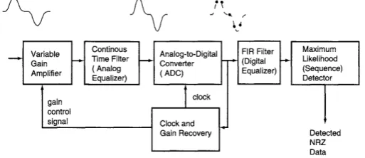
An example of the steps in the PRML is given in figure 2.2.

362 CHAPTER 12 PRML Channels

determined. A block diagram of a typical PRML channel is shown in Fig. 12.1. 7 It consists of a variable-gain amplifier (VGA), an analog equalizer, an analog-to-digital converter (ADC), a digital equalizer, an ML detector, and a clock/gain recovery circuit. The circuit blocks (except the ML detector) transform the readback signal into the partial response signal as required.

The analog readback signal from the magnetic head should have a certain and constant level of amplification. Any variation in isolated readback peaks is compensated with the VGA, which gets a control signal from the clock and gain recovery loop.

A PR channel operates within a certain bandwidth, meaning that the spectral components beyond the bandwidth have to be cut off. This is done with the continuous time filter or analog equalizer. The other function sometimes performed by the analog equalizer is to modify the frequency response of the channel. The modification of the frequency response is sometimes required to adjust the shape of the readback signal from the head. For example, it may be necessary to adjust the pulse width to make it proportional to the distance between transitions. The analog equalizer is implemented as a linear filter with a programmable frequency response including a variable cutoff frequency and boost. The analog signal at the equalizer output generally has a slightly different shape than the unmodified signal directly from the head.

The signal from the analog equalizer is sampled (or digitized) with the ADC. The sampling is initiated by a clock signal at the rate of exactly one sample per channel bit period. The frequency and phase of the clock

.•

Variable ~_~ Continous _Gain _{Time Filter} Amplifier ( Analog _Equalizer)

gain control signal

~.~ Analog-to-Digital _Converter ~ (ADC)

[image:13.595.147.404.431.542.2]

I clock I Cl~ ry ~'J

FIGURE 12.1. Block diagram of typical PRML channel.

Maximum Likelihood (Sequence) Detector Detected NRZ Data

Figure 2.2: Example of PRML, from [2]

2.2.4 Viterbi Detection

(14)

2.3

Two-dimensional techniques

2.3.1 M-Algorithm

The paper from Zadeh [3] describes a solution for a multitrack magnetic recording medium. In this description the input data is given as a two dimen-sional signal. In the channel model it is assumed there is only interference from adjacent tracks.

The several standard methods as Partial Response and Viterbi detectors are described, however, the problem with such detectors is the high number of states for only a small number tracks to be considered at one readout. The

M-Algorithm is a detector with a reduced complexity. From all paths theM

best paths are stored. An advantage of the M-algorithm over the Viterbi

Algorithm is the reduced number of paths, which makes it more suitable for longer paths and decreases the computations.

In Tosi [4] also a description for a system using the M-algorithm is given. This paper describes a partial response detection for a multi-track system.

2.3.2 Cross Talk Cancellation

In the thesis of Immink [5] the Cross Talk Cancellation (XTC) is discussed. With this technique three tracks are read out simultaneously and filtered versions of the two outer tracks are subtracted from the middle track in order to cancel the influence from the two outer tracks on the middle track. A quite simple method for improving the detection.

2.3.3 2D Viterbi Detection

The paper of Kato [7] to which is referred in Immink [5] has some interesting points about 2D Viterbi detection, but these are just seperated Viterbi detec-tors. The 2D viterbi detection described in Immink made some improvements on the Multitrack Viterbi Algorithm it is referring to. These refinements include taking into account weighing of contributions and taking into account other contributions.

Also non-linear ISI can be handled, by using the output of a previous calculated value of a state. The complexity of the algorithm has also been decreased.

2.3.4 Image Processing techniques

(15)

In chapter 5 more about these methods is given.

2.4

Patterned Media Solutions

Several papers are published about the two-dimensional detection in pat-terned media storage (PMS). An overview is given below.

2.4.1 Iterative Decision Feedback Detection

In Keskinoz [8] a description for a 2D detector for a patterned media is worked out in detail. The paper has 2 parts, one for a Iterative Decision Feedback Detection (IDFD) system and a 2D Generalized Partial Response (2D-GPR) with 1D Viterbi.

These techniques require more computations and have some requirements. IDFD requires all readings to be available to detect the information symbols. The 2D-GPR method performs better than IDFD under the same compu-tational load, whereas IDFD could achieve a higher SNR, employing more iterations.

2.4.2 Modifying Viterbi Algorithm

Nabavi [9] describes a modified version of the Viterbi Algorithm for bit-patterned media. This algorithm improves the BER while the complexity is not significantly increased. There are the same number of states, but the number of branches between these states increases.

The track misregistration (TMR) or read head offset is also taken into account, where as expected the modified Viterbi is more tolerant than the normal Viterbi.

2.5

Error Correction Codes

Errors will always occur in writing and reading data, due to noise and interference. To be able to correct errors, the user data is encoded with error correction codes (ECC).

Errors can occur in two types: single-bit errors and bursts of errors. A single-bit error can occur through a short noise event, which results in an extra pulse or a missing pulse. Bursts of errors usually occur through defects of the medium.

(16)

capacity of a medium can be improved with the ECC.

2.5.1 Low Density Parity Check codes

To improve the performance of the system, it is important to use a code which is optimized for the channel properties. Combinations of bits which are hard to detect have to be avoided in order to keep the error rate as low as possible.

The use of the right codes already inserts some redundancy in the bits stored on the media. In [10] several methods for the application of Low-Density Parity-Check (LDPC) codes are given, as well as the construction of optimal codes for different channel models.

A consequence on the use of complex coding is the complexity of the decoding that has to be done after the detection of the signal.

2.5.2 Run Length Limited codes

Run Length Limited (RLL) codes are codes which have a minimum and a maximum number of a value used after each other. For magnetic storage these values are a transition or no transition, a 1 or a 0. RLL Codes are typically referenced as (m/n)(d,k) codes. (m/n) Means: m user bits are

mapped onnencoded bits, wheren≥m. dis the minimum allowed number

of consecutive ”0”s between two ”1”s (d≥0). Andkis the maximum number

of consecutive ”0”s between two ”1”s (k≥0).

In the paper from Kato [7] a multi-track recording system with the use of 2D-PRML and 2D-RLL is described.

2.6

Methods in this work

While the storage medium in this work is in a exploratory status, the detection is started with a threshold detection on the two dimensional signal. Also two-dimensional versions of the peak detector and a decision feedback detector are applied.

A method using 3x3 samples per bit, which is designed within the TST-SMI group is implemented and some image processing techniques are applied on the signal and a comparison with the regular methods is made.

The results of the detectors are measured by the error rate of the detected bits. By varying the medium noise and the jitter on the medium, a comparison between the methods is made.

(17)

the input bits are applied. Only a simple coding method designed in the TST-SMI group is used for comparison with an uncoded situation. In this coding the worst-case patterns with bits of the same value are prevented from being present in the input signal. In every 3x3 bitpattern always one bit has value 1 and one bit is a 0.

(18)

(19)

Chapter

3

Detection on patterned media

Because of the exploratory status of this storage medium candidate, many design decisions have not been made yet. The readout of the signal might be influenced by changes in parts of the system. In order to perform the simulations, assumptions have been made which are described in this chapter.

3.1

Goal

The goal of this master assignment is to compare detection mechanisms on the aspects of medium noise and jitter. On the storage medium the bits are stored in a two-dimensional bit pattern. On conventional storage media the bits have only influence from the previous and next bit on the same track, the intersymbol interference (ISI). In a two-dimensional medium the bit patterns would have influence from the surrounding bits in two dimensions, so called 2D-ISI. Which is in fact an equivalent to Intertrack Interference (ITI) in conventional media.

Other important aspects in comparing detectors is the clocking problem. A clock-less detector, where bits are detected autonomously would be very practical. To be concurring with conventional storage media the information should be detected on a high speed, with a sample rate as low as possible and a high bit-density on the medium.

(20)

Chapter 3. Detection on patterned media

are necessary in order to reach a higher bit density. Every bit is stored on only 2 grains on the medium. The information across different tracks is used in the signal processing. The paper concludes that a fine grained medium is necessary in order to be able to reach the high density for 10 terabits per square inch and a practical two-dimensional detection scheme should be developed for detection of the bits with accurate timing and positioning.

In the next chapters various types of detection are described, including the conventional one-dimensional methods. Also techniques from the image processing field are taken into account, the signal can be seen as a picture with black and white dots on it. This can be described as an object recognition problem in image processing.

3.2

Properties of the MFM signal

The simulated signal is based on the experimental recording setup with a magnetic force microscope (MFM) from the TST-SMI group. It is in detail described in [12] and [13]. A CoNi/Pt multilayer is used as the recording medium and the periodicity of pulses goes down to 150 nm. The field is

scanned over the x and y direction. Writing the information is achieved

by approaching a MFM-tip to the medium in the presence of an external magnetic field in thezdirection. The read signal is a result from the vibrating MFM tip in the stray field of the magnetized dots. The signal is proportional to the second z derivative VM F M(x) ≈ (d2Hz(x)/dz2) integrated over the

tip volume.

The MFM signal can be simulated by a superposition of the individual MFM responses. When the individual pulses are written close to each other, the responses of these pulses overlap, influencing the output signal. This is the (two-dimensional) intersymbol interference which influences detection.

An example of a typical MFM output signal can be found in figure 3.1. It should be mentioned that while this image looks like a surface with dots on it, this is not how the recording medium surface looks like, but a result from the vibrating tip.

(21)

Figure 3.1: Output signal from MFM

3.3

Pulse description

3.3.1 One-dimensional

Rather than taking the full magnetostatic details into account, we can in first instance approximate the signal by a superposition of Lorentzpulses. This considerably speeds up calculation time. The Lorentz function is defined as

y= ₁₊1_x2. ISI is introduced by an overshoot of the pulse, also described by a

Lorentzpulse. The resulting pulse description for one bit is a combination of three Lorentzpulses:

pulse(x) = 3

X

i=1

vi

1 + ( x−xi

pw50i/2)

(3.1)

Where

vi = Amplitude of a Lorentz pulse

pw 50i = Lorentz pulse width, measured at 50% height ofvi

xi = Origin of the ith Lorentz.

A single pulse used in the simulations can be seen in figure 3.2.

3.3.2 Two-dimensional

The two-dimensional situation is just an expansion of the one-dimensional pulse from equation 3.1. The pulse is now described in two dimensions:

R=pX2₊_Y2

pulse(R) = 3

X

i=1

vi

1 + ( R−Ri

pw50i/2)

(22)

! "! #! $! %! &! '!

!!(# ! !(# !(% !(' !() " "(# *+,-.-+/ 0+1234-5678,-9/348:34;6 <_#

<_" <_$

=:61,>++. *?_&!

:_#

Figure 3.2: Single pulse

vi = Amplitude of a Lorentz pulse

pw 50i = Lorentz pulse width, measured at 50% height ofvi

Ri = Origin of the ith Lorentz.

In figure 3.3 an impression of this pulse description can be found.

5 10 15 20 25 30 35 40 5 10 15 20 25 30 35 40

(a) Image of 2 dimensional pulse

−30 −20 −10

0 10 20

−30 −20 −10 0 10 20 −0.2 0 0.2 0.4 0.6 0.8 1

(b) Spatial view of two-dimensional pulse

Figure 3.3: Two-dimensional pulse description.

In this pulse the overshoot around the pulse center can be seen, in figure 3.3(a) this overshoot is slightly darker than the surrounding. In the spatial view of figure 3.3(b) this overshoot can be seen as negative values.

(23)

3.4

Simulation parameters

3.4.1 Sample rate

The signal which will be used in the detectors is a sampled version of the MFM respons of the magnetic field. With a high sample rate there is a better description of the pulses on the medium, more samples are available per bit.

In simulations the sample rate is varied. From earlier work within the TST-SMI Group a sample rate of 3x3 samples per bit has been used in detection. The threshold detector uses only one sample per bit and for the remaining detectors also higher sample rates have been used for comparison of the detector performance on varying sample rates.

With higher sample rates more computation power is needed for the detection. Whether or not this is acceptable depends on the achieved gain in error rate.

3.4.2 Pulse period

The bits written on the medium are placed at some distance from each other, the pulse period. The description of the pulse is given in section 3.3. While varying the pulse period, also the influence from one pulse on the neighbouring pulses will vary. Specific patterns can have such an influence on surrounding pulses that bit values are hard to detect.

A small pulse period will result in a high bit density on the medium, while more errors will occur in detection. With a slightly larger distance between pulses the 2D-ISI will change. The error rate can be reduced and compensate for the loss in bit density. An optimum therefore will exist.

In figure 3.4 examples of pulse distances can be seen for a one dimensional signal. For a two-dimensional signal the same principle holds for both dimensions. These figures show a signal with two pulses of the same value. In case of two opposite values, the pulses will also influence, but increase the bit value of the neighbouring value, as is given in figure 3.5.

3.4.3 Pulse alignment

(24)

0 10 20 30 40 50 60 70 80

−0.2 0 0.2 0.4 0.6 0.8 1 1.2 Position

Normalized signal value

Period

(a) Big distance between

pulses

0 10 20 30 40 50 60 70

−0.2 0 0.2 0.4 0.6 0.8 1 1.2 Position

Period

(b) Small distance between pulses

! "! #! $! %! &! '! (! !!)# ! !)# !)% !)' !)* " ")# +,-./.,0 1,2345.6789-.:0459;45<7

(c) Combined signal of two pulses of fig 3.4(b)

Figure 3.4: Example of different pulse distances.

0 10 20 30 40 50 60 70

−1.5 −1 −0.5 0 0.5 1 1.5 Position

(a) Two opposite bit values

0 10 20 30 40 50 60 70

−1.5 −1 −0.5 0 0.5 1 1.5 Position

(b) Combined signal of bit val-ues

(25)

In figure 3.6 examples of the square and hexagonal pulse alignment can be found. With the use of a hexagonal alignment the distance between the rows is smaller, to keep the distance to the pulses in the neighbouring rows the same as the pulses on the same row.

20 40 60 80 100 120 140 160 180 200

20

40

60

80

100

120

140

160

180

200 (a) Square pulse alignment ₀ ₂₀ ₄₀ ₆₀ ₈₀ ₁₀₀ ₁₂₀ ₁₄₀ ₁₆₀ ₁₈₀ ₂₀₀

0

20

40

60

80

100

120

140

160

180

200 (b) Hexagonal pulse alignment

Figure 3.6: Square and hexagonal pulse alignment

3.4.4 Non-linearities of the read-out (perspective)

A typical output of the MFM, as can be seen in figure 3.1, shows a signal with pulses which are not equally spaced. For the detection now a localization problem arises. The pulses are not distributed homogeneous on the field. Solutions for this localization problems are a detector that finds the pulses autonomously. Without the knowledge of the position of the pulses the detector will find these pulses and the bit values. Another option is a transformation of the signal before detection is applied. In figure 3.1 the signal looks like a field with a perspective transformation. With a description of these non-linearities of the output signal a geometric transformation can be applied resolving the localization problem.

An example of a transformation can be found in figure 3.7. In figure 3.7(a) the original MFM output signal can be found. In figure 3.7(b) a rotation of 4 degrees is applied to the signal and in figure 3.7(c) a perspective transformation. The resulting image is a more homogeneous distribution of the pulses over the total field. During this transformations incomplete rows and colums are removed by cropping the image, this is indicated by the dashed lines in the figures.

(26)

Originele afbeelding

200 400 600 800 1000 1200

100 200 300 400 500 600 700 800 900 1000 1100

(a) MFM output signal

Rotated Image

100 200 300 400 500 600 700 800 900 1000 1100 100 200 300 400 500 600 700 800 900 1000

(b) MFM output after rota-tion

Transformed Image

100 200 300 400 500 600 700 800 900 1000 100 200 300 400 500 600 700 800 900 1000

(c) MFM output after per-spective transformation

Figure 3.7: Application of rotation and perspective transformation on MFM signal.

3.4.5 Borders

In the typical output signal of the MFM, given in figure 3.1, pulses are situated on the borders of the image. It is hard to detect these pulses, especially when transformation or filtering is applied on the signal. In the simulated signal this problem is solved by keeping the pulses a half pulse period from the border. Applying transformations does not result in disturbing the pulses on the borders.

A number of pulses situated on the border is also not taken into account in the calculation of the bit error rate (BER). The pulses on the borders are not surrounded by pulses on all sides and don’t have intersymbol interference from all sides. The detection for the bit values of these pulses usually will be easier compared to the pulses in the rest of the signal. The overhead of this border pulses will be two bits on all sides. With the current pulse description ISI and ITI will not have influence on more than two concurring neighbours.

3.4.6 Noise

Noise appears in different ways and can be divided in data dependent and data independent noise. The data dependent noise is in this work the ISI and ITI. With the use of an adapted detector or coding scheme this is noise which can be dealt with. The data independent noise can be divided into two types: Medium noise and Jitter.

Medium noise

(27)

every simulation this noise is varied to create a signal-to-noise ratio (SNR)/ bit error rate (BER) plot. A signal with a low SNR is given in figure 3.8(b). By looking at images of the signal dots are still detectable by the human eye, where for a detector the sample values might be below the given threshold value.

Jitter

Small misalignments in writing and reading the signal is called jitter. Dis-placement of the peaks of the pulses influences the detection. Jitter can be described as a noise on the position of each pulse. A detector should be able to detect the pulses while there is some jitter in the signal. An example of a signal disturbed by jitter can be found in figure 3.8(c). The pulses are not placed on the square raster, so the intersymbol interference will vary for all pulses.

In the simulations the jitter level is varied to compare the influence of it on the bit error rate of the detectors.

(a) Input signal without noise (b) Input signal with noise (c) Input signal with jitter

Figure 3.8: Examples of input signals used for detection

3.5

Error rate of the detection

In a 2D data storage system the goal is to reach a bit density as high as possible with a low error rate. We wish to store data at the highest possible density, without causing raw error rates above 10−4. A BER of 10−4 is chosen because error correction codes which will be applied after the detection are able to correct up to raw error rates of 10−4.

3.6

Clocking problem

(28)

detector that finds the pulses itself the knowledge of this information won’t be necessary and the problem with rotation and distortion doesn’t need to be solved before the detection is applied.

The detectors have been implemented with some boundary conditions. As input to the system a signal is given with a known number of written bits. The detectors assume the bits to be distributed homogeneous, which makes it possible to divide the signal in regions for every bit.

One of the problems in this autonomous detection is the noise influence on the signal. Extra pulses might occur or pulses become below threshold. The influence of jitter is a problem when the peaks are written close to each other, they might get written so close near each other that they won’t be distinguishable and will appear as just one pulse. This makes detection very difficult.

As a result from the 2D-ISI extra pulses might occur in the signal. A mechanism where a minimal distance is required between the samples of the detected bits can reduce the number of errors resulting from this influence.

The distortions visible in the output signal of the MFM influence the linear distribution of the pulses over the signal. The detection could compensate this by evaluating each detected pulse and adapt the expected pulse for the last few detected pulses. When the pulse period becomes wider this is compensated during detection and does not lead to an error. Such an error detection mechanism would cost extra computation power. Another possibility to compensate for the non-linearities is to apply transformation techniques. If the non-linearities of the MFM signal can be described this can be used for transformation.

(29)

Chapter

4

Detector description

This chapter describes the conventional detectors used for the simulations in this work. In appendix A the code for all detectors can be found. In the detectors the expected position of the pulses is assumed to be on a square pattern.

4.1

Threshold detector

The threshold detector checks whether the expected peakpoint of the field is above a certain threshold. An important parameter in this detector is the threshold value. With a high threshold the number of false positives due to noise is minimized. A low threshold value will give more influence from the noise. The threshold taken in the simulations is zero, exactly the middle between the positive and negative pulse values.

(a) Input signal without jitter and noise

(b) Input signal with jitter (c) Input signal with 5x5 bits of value 1

Figure 4.1: Threshold detector raster on three different signals.

(30)

Chapter 4. Detector description

be found. The sample values are the crossings of the dashed raster lines. In this figure errors occur, as a result from the intersymbol and intertrack interference.

This detector takes the value of the signal on fixed sample points, resulting in a lot of influence from jitter on it. This shift of peaks will result in lower sample values at the expected points. With high jitter, a sample value can be below threshold and the bit value will flip. In figure 4.1(a) and 4.1(b) an input signal without and with jitter can be seen, both with the same bit pattern. In figure 4.1(b) a lot of pulses are not on the expected peak points.

In the 5x5 bitpattern in figure 4.1(c) all bits have value one and the interfer-ence has such an influinterfer-ence on the bits in the center, that the values on the threshold detector will flip. The crossings of the raster lines in the figure are the sample points of the threshold detector.

4.2

Peak detector

The peak detector searches for a maximum in the expected peak window. A scheme of the steps in the peak detector can be found in figure 4.2.

By finding this maximum less influence from jitter is expected. Intersymbol interference and intertrack interference is the same as with the threshold detector. The interference can have such an influence that a positive peak will be flipped to a negative peak.

MFM Signal Output Bits

AND gate Differentiator

Rectifier

Zero crossing detector

Threshold detector

Figure 4.2: Schematic view of peak detector

In figure 4.3 and 4.5 the outputs of the steps of the peak detector applied on an MFM signal can be found. In figure 4.3 a large pulse period is used, figure 4.5 shows a smaller pulse period. The rectifier is applied, which transforms the signal to three values: -1, 0 and 1. The rectifier decides if a peak is high enough te be defined as a bit pulse or that it is a peak of the noisy background. The decision of the rectifier is based on a threshold value. The signal from the rectifier is given in figure 4.3(b).

(31)

of this two dimensional signal, the signal should be differentiated in both

x and y direction. If both differentiations have a zeros crossing, a local

maximum is detected. The combination of the rectified and differentiated signals completes the detection. A zero crossing of the differentiator indicates a maximum, or minimum, and a rectified signal of−1 or 1 defines if the peak is high enough to be assigned as a written pulse.

Instead of using the differentiations in both directions also the gradient can be used. The gradient of a two-dimensional signal is defined as:

∇f(x, y) =

"

∂f(x, y)

∂x

∂f(x, y)

∂y

#t

=

"

fx(x, y)

fy(x, y)

#

For each position the gradient points to the direction of the steepest ascent. And the magnitude k∇f(x, y)kis proportional to the steepness. In figure 4.4 the differentiations in both directions can be seen as well as the magnitude.mfmOutput

20 40 60 80 100 120 140

(a) MFM Output signal

20 40 60 80 100 120 140

(b) Rectified signal

differentiated output

20 40 60 80 100 120 140

(c) Differentiated signal

Figure 4.3: Signals of the steps of the peak detector with big pulse period

(a) Differentiation in X (b) Differentiation in Y (c) Magnitude of gradient

Figure 4.4: Differentiations in X and Y direction and magnitude

4.3

Triple detector

(32)

(a) MFM Output signal (b) Rectified signal (c) Differentiated signal

Figure 4.5: Signals of the steps of the peak detector with small pulse period

2D situation 3 samples for every dimension are taken, resulting in a signal with 3x3 samples per pulse. These samples are not depending on a clock.

In the one-dimensional situation a signal as in figure 4.6 is used. The signal is a sampled version of the continuous function in figure 4.6(a). For every pulse three samples are taken. Samples are indicated by the dashed lines and numbereds1. . . s9. For the first peak the sampless1, s2 ands3are compared.

Samples2 has the largest absolute value, indicated by a circle. Assuming

that the peak occurs in the center of three values, the next peak should occur in the samples s4, s5 and s6. For figure 4.6(a) the maximum is at sample

s5 and detection can continue for the last pulse. This will be detected on samples8.

In figure 4.6(b) jitter occurs on the signal. The second pulse is shifted. The maximum absolute value of the second pulse is no longer at samples5, but at samples4. For detection of the last pulse, the samples s6, s7 ands8 are taken into account. Samples6is hardly visible, the value is just on the x-axis. From these three sampless8 is the sample with the maximum absolute value.

If the signal from figure 4.6(b) consists of more pulses, the next samples for detection would bes10, s11 ands12. The pulse on sample s8 is assumed to be in the center of three samples, so samples9 is ignored.

Since three samples per bit are taken, the triple detector is theoretically insensitive to jitter. When the jitter misaligns the bits, as shown in figure 4.6(b), the triple detector will detect the maximum of that specific field in one of the other three samples.

(33)

0 10 20 30 40 50 60 70 80

−0.2 0 0.2 0.4 0.6 0.8 1 1.2 Position

(a) Detected values in jitterless case

0 10 20 30 40 50 60 70 80

−0.2 0 0.2 0.4 0.6 0.8 1 1.2 Position

(b) Detected values on signal with jitter

Figure 4.6: Triple detector samples on one dimensional signal.

to be examined are s(1,1) till s(3,3). From these 3x3 samples the absolute maximum is taken as the bit value.

The next 3x3 samples to be examined are based on the index of the detected maximum on the previous row and column, like in the 1D situation. In both the first row for they-samples always 1 till 3 are used, in the first column always thex-samples 1 till 3 are used. The detector is assumed to know the number of rows and columns of the bit pattern.

For this two-dimensional situation a 5x5 bitpattern is given in figure 4.7. Circles around the samples indicate a detected maximum. In figure 4.7(a) a jitterless signal is given and the peaks are detected on the raster. In figure 4.7(b) a signal highly influenced by jitter is given, the detected maxima are indicated by the circles.

The performance of the triple detector depends a lot on the initial settings of the detector. A change in resolution or distance between peaks without adapting the sample rate will influence the performance. The startpoint of the signal should be defined clearly, having the first signal peak within the first three samples. If the first value is detected wrong this might result in an error burst, causing a high bit error rate due to an error propagation. The detected bits might be right, but shifted in one or more places.

(34)

(a) Detected values (b) Detected values on signal with high jitter

Figure 4.7: Triple detector samples on two dimensional signal.

4.4

Decision Feedback Equalization

The decision feedback equalization (DFE) is an iterative detection method where the influence from one pulse to the surrounding pulses, the 2D-ISI, is taken into account. With an approximation of the pulse written on the medium, this (expected) interference can be removed from the surrounding pulses. Specific bitpatterns will result in highly influenced pulses by the interference of neighbouring pulses. Pulses might be cancelled or even flipped, which can be seen in figure 4.1(c). The cancellations will be reversed with this detector, making detection of bits in highly influenced signals possible.

The DFE detector used in this work is a two-dimensional implementation of the DFE described in Wang [2]. An implementation of a two-dimensional DFE can also be found in the paper of Keskinoz [8].

In figure 4.8 a schematic view of the DFE can be found. The decision block detects the value of a pulse on the expected peak point of the pulse and uses this value for the pulse description to be subtracted from the signal. With the removal of a pulse, also the 2D-ISI is removed from the surrounding pulses. Now detection can be continued for the next pulse.

(35)

Input

Output

Decision Pulse Description

!

+

-Figure 4.8: Schematic view of DFE

In a 1D situation the signal, as a function of the time, is as given in figure 4.9. Three pulses with ISI are given as the input signal. The removal of the expected pulse from the input signal, makes the next pulse better distinguishable, as can be seen in figure 4.9(b) and 4.9(c).

0 10 20 30 40 50 60

−0.4 −0.2 0 0.2 0.4 0.6 0.8 1 time amplitude

(a) Input signal

0 10 20 30 40 50 60

−0.4 −0.2 0 0.2 0.4 0.6 0.8 1 time amplitude

(b) Removal of first pulse

0 10 20 30 40 50 60

−0.4 −0.2 0 0.2 0.4 0.6 0.8 1 time amplitude

(c) Removal of second pulse

Figure 4.9: DFE detector on 1D signal.

For the 2D signal the situation is similar. In figure 4.10 the steps of the detector can be seen. A signal with a 5x5 bit pattern is used, where all bits are a one (which was also shown by the threshold detector in figure 4.1(c)). Figure 4.10(a) is the input signal of the detector. In figure 4.10(b) the pulses of the first row are subtracted from the signal, removing also the influence from these pulses on the surrounding pulses in the next row. This makes the pulses towards the center better distinguishable. In figure 4.10(c) two more pulses are removed and in figure 4.10(d) the signal is given just before the detection of the pulse in the center.

By comparing figure 4.10(a) with figure 4.10(d) it can be seen that the center value of this 5x5 bit pattern is detected correctly with the DFE detection. In case of a threshold or peak detection this value would be detected wrong due to 2D-ISI of the surrounding pulses.

(36)

(a) Input signal (b) After first row removal

(c) After two more pulse removals (d) Detection of center pulse

(37)

on a slightly different position than the pulse actually occurs in the signal. The influence on neighbouring pulses will not be removed the way it has influenced these neighbours during writing. There will be influence of jitter on the performance of this detector.

In figure 4.11 the same detection is applied as in figure 4.10, now on a signal with jitter. It can be seen in figure 4.11(d) that after removal of pulses a more noisy signal is left, a result of the remaining ISI. The pulses are removed from the expected peak point, but due to jitter the written pulses are shifted and the influence from ISI is also different than expected.

(a) Input signal (b) After first row removal

(c) After two more pulse removals (d) Detection of center pulse

Figure 4.11: DFE detector signal during several detection steps, with jitter influence.

4.5

Detectors on patterned media

(38)

3.1. By varying the pulse period, signal to noise ratio, jitter and sample rate comparisons can be made between the performances of these detectors. The results of these simulations are given in chapter 6.

(39)

Chapter

5

Image Processing Techniques

In all methods described in chapter 4 impressions of the signal are shown as grayscale images. On these images dots appear and depending on the presence of noise and jitter, these dots are more or less distinguishable. Instead of using the common detection methods derived from the one-dimensional methods, specific image processing recognition and detection methods can be used. The dots can be detected with object recognition algorithms and so the bit values of the input signal can be detected.

The MFM signal is built of positive and negative pulses with more or less known properties. These pulses are the objects to be recognized and appear as black and white dots on a gray background. The geometry of the pulses is rotational invariant.

Different methods from the book Image Based Measurement Systems by Van der Heijden[16] are applied on the simulation of the MFM signal and described in the next sections.

5.1

Spot Detection

In the signal generated in the simulation, the dots are clearly visible when displayed as an image. From an image processing view this looks like a spot detection problem. A model for the description of the spot field is given in equation 5.1.

f(x, y) =C0+

X

i

(40)

Chapter 5. Image Processing Techniques

In this equation C0 is the background and Cih are the amplitudes of the

spots on the respective (xi, yi) positions. The goal is to detect the positions

of the spots in thef(x, y) image, in which the Ci value is the value of this

bit, either−1 or 1.

It is a very obvious way to detect these pulses by comparing the image with a template. The template is a description of the image to be detected. A cross correlation can be calculated between the input image and the template. This cross correlation information can be used in a detector where values on specific positions will exceed a threshold, defining the position of the spot.

In terms of image processing the process for the spot detection now exists of two parts: Feature extraction and classification.

5.2

Feature extraction

Goal of the algorithms is finding the dots in the image. These dots have certain properties, called features. By extracting these features from the MFM signal, and so reducing the disturbances in the signal, the relevant information is left over for detection.

5.2.1 Point spread function

The point spread function (PSF) of the pulses is described in chapter 3 as the pulse description of the simulation signal. This same function can be used in the image processing detection mechanisms for comparison with the input signal. The resolution of the PSF is depending on the resolution of the dots in the MFM signal. An example of the PSF and the associated matrix is given in figure 5.1.

5.2.2 Euclidean Distance

By comparing the MFM signal with a template, a distance can be calculated between these two signals. The position of the template on the signal with the smallest distance is the expected position for a peak. This comparison can be done with the euclidean distance between the image and the template. The calculation for the distance is given in equation 5.2.

d2(ξ, η) =

Z Z

x,y

(f(x, y)−h(x−ξ, y−η))2 d( ˆξ,ηˆ) = min{d(ξ, η)} (5.2)

Which can be written as

d2(ξ, η) =

Z Z

x,y

(f(x+ξ, y+η)−h(x, y))2 (5.3)

(41)

(a) Full pulse description (b) Pulse part of interest

(c) Associated matrix

     

−0.06 0.11 0.21 0.11 −0.06

0.11 0.50 0.72 0.50 0.11 0.21 0.72 1.00 0.72 0.21 0.11 0.50 0.72 0.50 0.11

−0.06 0.11 0.21 0.11 −0.06

     

Figure 5.1: Example of PSF description

dn,m =d(n∆, m∆). In equation 5.2 and 5.4f is the MFM signal and h is

the template image, the description of the pulse in the absence of noise. The

constants K andL should be chosen such that the template image covers

the whole object of interest, in this specific case the size of a single dot in the MFM signal.

d2_n,m =

K

X

k=−K

L

X

l=−L

(fn+k,m+l−hk,l)2 (5.4)

With a template image as close as possible to the written pulse and an input signal with no 2D-ISI the distance will be minimal and approach zero. The 2D-ISI and medium noise will influence the euclidean distance and jitter will change the location of the minimum. An example of the euclidean distance of an input signal to a template is given in figure 5.2. A noisy input signal gives an enhanced output which can be used in the classification step.

(42)

(a) Noisy MFM signal (b) Euclidean distance to

pos-itive peak

(c) Euclidean distance to neg-ative peak

Figure 5.2: Application of euclidean distance on MFM signal

5.2.3 Convolution

Convolution of the signal with the mathematical description of a pulse is an equivalent of matched filtering. In this detector the signal is convoluted with the PSF.

The operation is a weighted sum of signal levels from a region of the signal. The weight factors are the samples of the pulse description. The matrix of weight factors is called the convolution maskh, which is in fact a template image. With a convolution mask that matches the pulses coming from the MFM signal, the weighted sum is maximized on the location where the pulses exist in the MFM signal. After this convolution the pulses will be enhanced and noise will be suppressed. This method is also called linear image filtering: an input signal is lowpass filtered with the description of the expected objects in this input signal.

The convolution can be mathematically described as equation 5.5. The

detector starts with the signal fn,m and this signal is convoluted with a

convolution mask,hn,m. Both are matrices and with the inner product the

values for the convoluted signal gn,m results.

gn,m=h’f= K

X

k=−K

L

X

l=−L

hk,lfn−k,m−l=hn,m∗fn,m (5.5)

Convolution masks

(43)

will be visible, for example the undershoot of the pulse, which is overlapping with the neighbouring pulses. An adapted convolution mask can give similar results with a reduced number of calculations.

A gaussian pulse can be used as a convolution mask. In equation 5.6 the description for a gaussian pulse is given.

hx,y =Ae −

(x−x0)2

2σ2x +

(y−y0)2 2σ2y

(5.6)

WhereA is the amplitude of the pulse. x0 and y0 the centers of the pulse and σx and σy the xand y spreads.

This pulse as convolution mask can easily be adapted from a circular to elliptical form by using different values forσxandσy. Examples of convolution

masks created by a gaussian pulse are given in figure 5.3. In figure 5.3(c) also a rotated mask can be found. In case of the typical MFM signal example given in section 3.4.4 this mask can be used before rotation and transformation of the signal is applied.

(a) Circular Gaussian convo-lution mask

(b) Elliptical convolution

mask

(c) Rotated elliptical convolu-tion mask

Figure 5.3: Examples of convolution masks

Applying convolution masks

In figure 5.4 the output signals can be found after applying various convolution masks. The MFM signal is given in figure 5.4(a). After convolution with an 8x8 mask of the pulse description of section 3.3.2 the output is given in figure 5.4(b). Figure 5.4(c) shows the output after convolution with a gaussian description for the convolution mask as a 5x5 matrix.

(44)

In figure 5.5 the result of applying convolution on a noisy MFM signal with a bit pattern of 5x5 ones can be found. The output after convolution is given in figure 5.5(b). The black dots that occur as a result of the 2D-ISI still exist and may cause problems in the classification.

(a) Simulated MFM Output signal

(b) Convolution with pulse de-scription

(c) Convolution with gauss pulse

Figure 5.4: Applying different convolution masks

(a) Noisy MFM signal of 5x5 ones (b) Convolution output of 5x5 ones

Figure 5.5: Applying convolution on noisy 5x5 ones

Image border effects

When a convolution is applied, there will occur irregularities on the borders. An example can be seen in figure 5.6. In figure 5.6(b) a disturbance of the bits on all borders is visible.

(45)

has been applied and pulses on the borders are not disturbed by the border effect anymore.

20 40 60 80 100 120 140 160 180 200

20

40

60

80

100

120

140

160

180

200 (a) Simulated MFM Output

signal

20 40 60 80 100 120 140

20

40

60

80

100

120

140

(b) Convolution without

padding with zero’s 20 40 60 80 100 120 140 160 180 200

20

40

60

80

100

120

140

160

180

200 (c) Convolution with padding

Figure 5.6: Border effects with convolution

5.2.4 Laplacian of the Gaussian

On the signal after convolution the Laplace operator can be applied. The Laplacian is the second order derivative, given in equation 5.7.

∆f =∇2f = δ 2_f

δx2 +

δ2f

δy2 (5.7)

The result of this operator on a signal after convolution is a strong respons on the positions for the black and white dots on the MFM signal. In figure 5.7(b) the result of this operator applied on figure 5.7(a) can be found.

(a) Convoluted MFM signal (b) After application of Laplacian

(46)

5.3

Classification

After the feature extraction methods the dots in the signal are enhanced. The next step is to localize the dots in the signal and decide whether or not they are a written pulse or a result of ISI and ITI.

5.3.1 Non-local maximum suppression

Besides a way of detecting pulses, there is also the problem of the localization of the pulses. In an ideal situation the detector should be able to localize the pulses, making the use of a clock unnecessary. A non-local maximum suppression algorithm is a method for solving this problem. As the name says, it is a suppression of the non-local maxima. At the output of this algorithm the local maxima are still available, representing the pulses of the signal. With this algorithm the influence of jitter is also minimized.

In the MFM signal, matrix f, there are positive and negative peaks. To

make all dots positive the absolute value of the signal is taken, resulting

infabs. Now for all samples in the signal a comparison can be made with

the neighbouring values. When a sample is larger than the samples in its direct surrounding and above the threshold value, the position is classified

as a peak. The output matrixfout now consists of values −1 or 1 on peak

positions and 0 elsewhere. The algorithm of this method is given in listing 5.1.

f _ a b s = abs ( f );

f _ o u t = z e r o s ( s i z e ( f )); t h r e s h o l d = THD ;

for i = 1: r o w S a m p l e s for j = 1: c o l S a m p l e s

if ((( f _ a b s ( i , j ) >= f _ a b s ( i -1 , j )) && ... ( f _ a b s ( i , j ) >= f _ a b s ( i +1 , j )) && ... ( f _ a b s ( i , j ) >= f _ a b s ( i , j - 1 ) ) && ... ( f _ a b s ( i , j ) >= f _ a b s ( i , j + 1 ) ) ) && ... ( f _ a b s ( i , j ) >= f _ a b s ( i -1 , j - 1 ) ) && ... ( f _ a b s ( i , j ) >= f _ a b s ( i +1 , j + 1 ) ) && ... ( f _ a b s ( i , j ) >= f _ a b s ( i +1 , j - 1 ) ) && ... ( f _ a b s ( i , j ) >= f _ a b s ( i -1 , j + 1 ) ) ) if ( f _ a b s ( i , j ) > t h r e s h o l d ))

f _ o u t ( i , j ) = s i g n ( f ( i , j )); end

e l s e

f _ o u t ( i , j ) = 0; end

end end

(47)

The number of samples in the surrounding which is taken into account can be varied. Depending on the size, the sample rate and the period of the dots on the signal.

The result of applying this algorithm to the signal after convolution is given in figure 5.8. In 5.8(a) the convolution output is given, which results in figure 5.8(b) after the algorithm. An input signal with noise can be found in figure 5.9. In that case more local maxima appear, which results in extra positive and negative samples.

In figure 5.8(b) also the effects of 2D-ISI are visible. In the output extra local maxima appear. The 2D-ISI introduces extra peaks. For example the extra white dot between the black dots in the upper left 3x3 bits. To prevent the algorithm from classifying these effects the first step is to change the threshold. When the 2D-ISI is such that the interference peak will be higher than a written pulse, this won’t work. This can be seen in figure 5.10 where in input signal with 5x5 ones is used. The output after non-local maximum suppression in figure 5.10(b) shows extra detected pulses due to the 2D-ISI. A solution would be to require a minimal distance between the position of detected peaks.

(a) Input signal (b) Output after non-local maximum

suppression algorithm

Figure 5.8: Application of non-local maximum suppression algorithm.

5.4

Image processing on patterned media

(48)

(a) Input signal (b) Output after non-local maximum

Figure 5.9: Application of non-local maximum suppression algorithm on noisy signal.

(a) MFM signal of 5x5 ones (b) Output after non-local maximum

(49)

Chapter

6

Results and Discussion

This chapter gives the results of the different detectors with different influence from jitter and medium noise. The simulations are done with the pulse description given in chapter 3 with an input matrix of 25x25 bits. The signal is simulated with varying sample rates and pulse periods. On the borders the pulses are not influenced from all sides, as described in section 3.4.5. By removing two bits on all sides a number of databits of 23x23 bits is used in each simulation signal. This signal is generated many times with a pseudorandom bitpattern.

In conventional storage media a raw bit error rate of 10−4 is the maximum for a detector to be useful in detection. For the simulations in this work this is also the guideline. If in a series of simulations no errors occur this doesn’t mean the bit error rate is zero. It just means that not enough bits are simulated to detect the errors. However, also detecting only a few errors with a big number of simulations is no measurement for a low BER. Before the BER is statistically significant at least 100 errors have to be detected. This means for a statistically significant BER of 10−4 at least one million bits have to be simulated.

6.1

Patterned media simulations

(50)

Chapter 6. Results and Discussion

signal can be found. A 5x5 bit pattern is generated for different distances and SNR values.

(a) SNR = 0dB (b) SNR = 4dB (c) SNR = 8dB

(d) SNR = 0dB (e) SNR = 4dB (f) SNR = 8dB

Figure 6.1: Signal examples for different distances and SNR values. (a) - (c) - distance 7 samples, (d)-(f) - distance 9 samples.

By using a larger distance between the pulses the influence of the 2D-ISI on the signal can be compared. The result of these simulations with influence of jitter and medium noise is given below.

6.1.1 Jitter Influence

Jitter can be described as noise on the position of the pulses. Especially the detectors where the sample value on the expected points is used could suffer from this noise. The jitter will also change the 2D-ISI, some pulses will be closer together than others. In figure 6.2 the bit error rates (BER) for the different detectors can be found.

In figure 6.2(a) it can be seen that the threshold detector (THD) has the highest BER. The convolution improves the detection of the pulses and performs the best. Up to a jitter of 0.6 the BER of 10−4 is still feasible.

(51)

0 0.1 0.2 0.3 0.4 0.5 0.6 0.7 0.8 0.9 1 10−7

10−6 10−5 10−4 10−3 10−2 10−1

Jitter

BER

THD DFE Convolution

(a) Peak distance = 9

0 0.1 0.2 0.3 0.4 0.5 0.6 0.7 0.8 0.9 1

10−7 10−6 10−5 10−4 10−3 10−2 10−1 Jitter BER THD DFE Convolution

(b) Peak distance = 8

Figure 6.2: Detector performance by jitter influence for SNR = 4.

6.2(b).

0 0.1 0.2 0.3 0.4 0.5 0.6 0.7 0.8 0.9 1 10−7 10−6 10−5 10−4 10−3 10−2 10−1 Jitter BER THD DFE Convolution

(a) Peak distance = 9

0 0.1 0.2 0.3 0.4 0.5 0.6 0.7 0.8 0.9 1

10−7 10−6 10−5 10−4 10−3 10−2 10−1 Jitter BER THD DFE Convolution

(b) Peak distance = 8

Figure 6.3: Detector performance by jitter influence for SNR = 0.

In figure 6.3 the results of the detectors in the presence of more noise, a lower SNR, is given. As expected the convolution will perform better than the other detectors. The noise influence is filtered out and the detector is still able to detect the bits successfully, while the threshold and DFE will have much more errors.

6.1.2 Medium Noise Influence

(52)

same behaviour as can be seen in the jitter plots. The performance won’t get better above a certain SNR, due to the worst-case patterns in the signal.

0 2 4 6 8 10 12 14 16 18 20

10−7 10−6 10−5 10−4 10−3 10−2 10−1 SNR (dB) BER THD DFE Convolution

(a) Pulse distance = 8

0 2 4 6 8 10 12 14 16 18 20

10−7 10−6 10−5 10−4 10−3 10−2 10−1

SNR (dB)

BER

THD DFE Convolution

(b) Pulse distance = 7

Figure 6.4: Detector performance by medium noise.

6.1.3 Pulse distance

With a variation in the pulse period the influence of 2D-ISI can be examined. In figure 6.5 the BER for a varying period can be found. Each pulse is simulated with 15x15 samples and the peaks of the pulses are placed on a distance of 7 to 11 samples. The BER is given for a SNR of 0 and 4 dB. The pulse which is given in section 3.3.2 is used in the simulations.

In the situation of a distance of 7 samples, the peak of a pulse is exactly on the overshoot peak of a neighbouring pulse. With this maximal 2D-ISI it is expected that detectors suffer from this. As could also be seen in figure 6.4(b) the DFE will perform the best on a small pulse distance, on a higher SNR. In that case the convolution cannot distinguish the pulses.

6.1.4 Lower sample rate

In the previous results the sample rate was 15x15 samples per individual pulse. Also a lower sample rate is simulated. With a sample rate of 7x7 samples per pulse and a pulse distance of 4 samples a signal is generated with 3x3 samples per bit. With a pulse distance of 5 samples a signal with 4x4 samples per bit is generated. On both signals also the triple detector is applied.

(53)

7 7.5 8 8.5 9 9.5 10 10.5 11

10−7

10−6

10−5 10−4

10−3

10−2 10−1

Peak Distance

BER

THD DFE Convolution

(a) SNR = 0

7 7.5 8 8.5 9 9.5 10 10.5 11

10−7 10−6 10−5 10−4 10−3 10−2 10−1 Peak Distance BER THD DFE Convolution

(b) SNR = 4

Figure 6.5: Detector performance for change in distance.

other detectors. Only for SNR = 0 dB a BER around 10−3 can be seen.

The result of a simulation with a sample rate of 3x3 samples per bit can be seen in figure 6.6(b). For both the triple and the convolution detector the BER won’t get better above a SNR around 20 dB.

0 5 10 15 20 25 30

10−6 10−5

10−4 10−3

10−2

10−1 100 SNR (dB) BER THD Trio DFE Convolution

(a) 4x4 samples per bit

0 5 10 15 20 25 30

10−6

10−5

10−4

10−3

10−2

10−1

100 SNR (dB) BER THD Trio DFE Convolution

(b) 3x3 samples per bit

Figure 6.6: Detector performance for different samples per bit.

(54)

Figure 6.7(b) points out that the DFE is able to reach the best BER in case of jitter.

0 5 10 15 20 25 30

10−6 10−5 10−4 10−3 10−2 10−1 100 SNR (dB) BER THD Trio DFE Convolution

(a) 4x4 samples per bit

0 5 10 15 20 25 30

10−6

10−5

10−4

10−3

10−2

10−1

100 SNR (dB) BER THD Trio DFE Convolution

(b) 3x3 samples per bit

Figure 6.7: Detector performance for different samples per bit with jitter.

6.1.5 Simple coding

In the paper of Groenland [11] a simple coding scheme is introduced. In this coding scheme the signal is prevented from the occurence of worst-case patterns where ISI of neighbouring pulses will cancel out one pulse. In a 3x3 bit pattern always one bit has value 1 and one bit has value 0.

In figure 6.8 the uncoded signal with the threshold, DFE and convolution detector is compared with the coded signal of the threshold detector of the paper. For this specific coding method the signal simulation of the paper of Groenland [11] has been used.

Due to a slightly different description of the pulses in the simulation of the paper there is a performance difference in comparison to figure 6.6. All detectors in figure 6.8 are applied on the pulse description from the paper. It can be seen that a coded signal on the threshold detector improves detection, but still the DFE and convolution in an uncoded situation perform better.

6.2

Triple detector

Special attention is given to the triple detector. The performance of the detector is disappointing, so some analysis is done on the signal to get more information about the situation where detection is unsuccessful.

(55)

0 0.05 0.1 0.15 0.2 0.25 0.3 0.35 10−4

10−3

10−2 10−1

Jitter

bER

bit error rate for uncoded and coded THD signal

THD THD Uncoded DFE Convolution

Figure 6.8: Jitter influence on threshold, DFE and convolution detection with coded input signal for THD

right, which can be seen from the circles around the detected samples in figure 6.9(a).

(a) Input signal (b) Detected samples

Figure 6.9: Triple detector on 5x5 bits pattern with 3x3 samples per bit.

In figure 6.10 the signal of a bit pattern with all ones can be seen. The ISI and ITI is very large and the peaks between the bit pulses are detected as maximal values. This is the wrong value and a lot of errors occur. In simulations of a larger signal with random bit values also patterns will occur with 3x3, or even more, bits of the same value.

(56)

Figure 6.10: Triple detector on 5x5 bits pattern with all ones.

a error burst, because the next detected pulses are shifted one position.

Figure 6.11: Triple detector on 5x5 bits pattern with high jitter.

In figure 6.12 a signal with more pulses is generated. The detected pulses are nicely ordered on a raster, but on the seventh row an error occurs. All other rows have 4 samples, and this row only 3. Now all next pulses on that row are shifted one position. The detected pulses are right, but on the wrong position and this results in a difference between the input and output bitstream.

(57)

(58)

(59)

Chapter

7

Conclusions and

Recommendations

7.1

Conclusions

Different detectors have been investigated on random patterns with jitter and medium noise. The error rates of the detectors have been compared resulting in the following conclusions.

7.1.1 Detector performance

For the situation with jitter on the received signal, the decision feedback equal-ization and convolution detectors perform better than the simple threshold detector. The threshold detector always will have errors due to the worst-case patterns, where a pulse is surrounded by pulses of the same sign. This presence of those patterns is of less influence with the other detectors. In the DFE the influences from s

Two dimensional coding and detection for data storage on patterned media

Master Thesis

Contents

CONTENTS

CONTENTS

Chapter

Chapter

One-dimensional techniques

Two-dimensional techniques

Patterned Media Solutions

Error Correction Codes

Methods in this work

Chapter

Properties of the MFM signal

Pulse description

Simulation parameters

Error rate of the detection

Chapter

Peak detector

Triple detector

Decision Feedback Equalization

Input

Detectors on patterned media

Spot Detection

Feature extraction

Classification

Image processing on patterned media

Patterned media simulations

Triple detector

Chapter