Bounding and Comparing Methods for Correlation Clustering Beyond ILP

Bounding and Comparing Methods for Correlation Clustering Beyond ILP

Micha Elsner and Warren Schudy Department of Computer Science

Brown University Providence, RI 02912

{melsner,ws}@cs.brown.edu

Abstract

We evaluate several heuristic solvers for corre-lation clustering, the NP-hard problem of par-titioning a dataset given pairwise affinities be-tween all points. We experiment on two prac-tical tasks, document clustering and chat dis-entanglement, to which ILP does not scale. On these datasets, we show that the cluster-ing objective often, but not always, correlates with external metrics, and that local search al-ways improves over greedy solutions. We use semi-definite programming (SDP) to provide a tighter bound, showing that simple algorithms are already close to optimality.

1 Introduction

Correlation clustering is a powerful technique for discovering structure in data. It operates on the pairwise relationships between datapoints, partition-ing the graph to minimize the number of unrelated pairs that are clustered together, plus the number of related pairs that are separated. Unfortunately, this minimization problem is NP-hard (Ailon et al., 2008). Practical work has adopted one of three strategies for solving it. For a few specific tasks, one can restrict the problem so that it is efficiently solv-able. In most cases, however, this is impossible. In-teger linear programming (ILP) can be used to solve the general problem optimally, but only when the number of data points is small. Beyond a few hun-dred points, the only available solutions are heuristic or approximate.

In this paper, we evaluate a variety of solu-tions for correlation clustering on two realistic NLP

tasks, text topic clustering and chat disentangle-ment, where typical datasets are too large for ILP to find a solution. We show, as in previous work on consensus clustering (Goder and Filkov, 2008), that local search can improve the solutions found by commonly-used methods. We investigate the rela-tionship between the clustering objective and exter-nal evaluation metrics such as F-score and one-to-one overlap, showing that optimizing the objective is usually a reasonable aim, but that other measure-ments like number of clusters found should some-times be used to reject pathological solutions. We prove that the best heuristics are quite close to op-timal, using the first implementation of the semi-definite programming (SDP) relaxation to provide tighter bounds.

The specific algorithms we investigate are, of course, only a subset of the large number of pos-sible solutions, or even of those proposed in the lit-erature. We chose to test a few common, efficient algorithms that are easily implemented. Our use of a good bounding strategy means that we do not need to perform an exhaustive comparison; we will show that, though the methods we describe are not per-fect, the remaining improvements possible with any algorithm are relatively small.

2 Previous Work

Correlation clustering was first introduced by Ben-Dor et al. (1999) to cluster gene expression pat-terns. The correlation clustering approach has sev-eral strengths. It does not require users to specify a parametric form for the clusters, nor to pick the number of clusters. Unlike fully unsupervised

tering methods, it can use training data to optimize the pairwise classifier, but unlike classification, it does not require samples from the specific clusters found in the test data. For instance, it can use mes-sages about cars to learn a similarity function that can then be applied to messages about atheism.

Correlation clustering is a standard method for coreference resolution. It was introduced to the area by Soon et al. (2001), who describe the first-link heuristic method for solving it. Ng and Cardie (2002) extend this work with better features, and de-velop the best-link heuristic, which finds better solu-tions. McCallum and Wellner (2004) explicitly de-scribe the problem as correlation clustering and use an approximate technique (Bansal et al., 2004) to enforce transitivity. Recently Finkel and Manning (2008) show that the optimal ILP solution outper-forms the first and best-link methods. Cohen and Richman (2002) experiment with various heuristic solutions for the cross-document coreference task of grouping references to named entities.

Finally, correlation clustering has proven useful in several discourse tasks. Barzilay and Lapata (2006) use it for content aggregation in a generation system. In Malioutov and Barzilay (2006), it is used for topic segmentation—since segments must be contiguous, the problem can be solved in polynomial time. El-sner and Charniak (2008) address the related prob-lem of disentangprob-lement (which we explore in Sec-tion 5.3), doing inference with the voting greedy al-gorithm.

Bertolacci and Wirth (2007), Goder and Filkov (2008) and Gionis et al. (2007) conduct experiments on the closely related problem of consensus

ing, often solved by reduction to correlation

cluster-ing. The input to this problem is a set of clusterings; the output is a “median” clustering which minimizes the sum of (Rand) distance to the inputs. Although these papers investigate some of the same algorithms we use, they use an unrealistic lower bound, and so cannot convincingly evaluate absolute performance. Gionis et al. (2007) give an external evaluation on some UCI datasets, but this is somewhat unconvinc-ing since their metric, the impurity index, which is essentially precision ignoring recall, gives a perfect score to the all-singletons clustering. The other two papers are based on objective values, not external

metrics.1

A variety of approximation algorithms for corre-lation clustering with worst-case theoretical guar-antees have been proposed: (Bansal et al., 2004; Ailon et al., 2008; Demaine et al., 2006; Charikar et al., 2005; Giotis and Guruswami, 2006). Re-searchers including (Ben-Dor et al., 1999; Joachims and Hopcroft, 2005; Mathieu and Schudy, 2008) study correlation clustering theoretically when the input is generated by randomly perturbing an un-known ground truth clustering.

3 Algorithms

We begin with some notation and a formal definition of the problem. Our input is a complete, undirected graph Gwith nnodes; each edge in the graph has a probabilitypij reflecting our belief as to whether

nodesiandjcome from the same cluster. Our goal is to find a clustering, defined as a new graph G′ with edges xij ∈ {0,1}, where if xij = 1, nodes

iand j are assigned to the same cluster. To make this consistent, the edges must define an equivalence relationship: xii = 1 and xij = xjk = 1 implies

xij =xik.

Our objective is to find a clustering as consistent as possible with our beliefs—edges with high proba-bility should not cross cluster boundaries, and edges with low probability should. We definew+_ij as the cost of cutting an edge whose probability ispij and

w−_ij as the cost of keeping it. Mathematically, this objective can be written (Ailon et al., 2008; Finkel and Manning, 2008) as:

min X ij:i<j

xijw_ij−+ (1−xij)w_ij+. (1)

There are two plausible definitions for the costsw+ andw−, both of which have gained some support in the literature. We can take w_ij+ = pij and w−ij = 1−pij (additive weights) as in (Ailon et al., 2008)

and others, or w_ij+ = log(pij), w−ij = log(1−pij)

(logarithmic weights) as in (Finkel and Manning, 2008). The logarithmic scheme has a tenuous math-ematical justification, since it selects a maximum-likelihood clustering under the assumption that the

pij are independent and identically distributed given

the status of the edge ij in the true clustering. If we obtain thepij using a classifier, however, this

as-sumption is obviously untrue—some nodes will be easy to link, while others will be hard—so we eval-uate the different weighting schemes empirically.

3.1 Greedy Methods

We use four greedy methods drawn from the lit-erature; they are both fast and easy to implement. All of them make decisions based on the net weight w±_ij =w_ij+₋w−_ij.

These algorithms step through the nodes of the graph according to a permutationπ. We try 100 ran-dom permutations for each algorithm and report the run which attains the best objective value (typically this is slightly better than the average run; we dis-cuss this more in the experimental sections). To sim-plify the pseudocode we label the vertices1,2, . . . n in the order specified by π. After this relabeling π(i) = iso π need not appear explicitly in the al-gorithms.

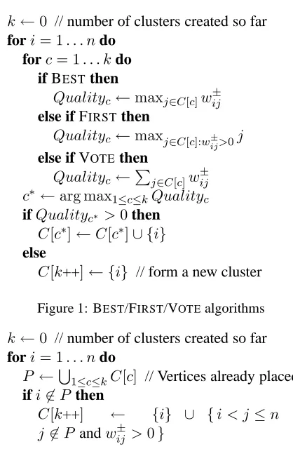
Three of the algorithms are given in Figure 1. All three algorithms start with the empty clustering and add the vertices one by one. The BEST algorithm adds each vertex ito the cluster with the strongest w±connecting toi, or to a new singleton if none of thew±are positive. The FIRSTalgorithm adds each vertex ito the cluster containing the most recently considered vertexjwithw_ij± >0. The VOTE algo-rithm adds each vertex to the cluster that minimizes the correlation clustering objective, i.e. to the cluster maximizing the total net weight or to a singleton if no total is positive.

Ailon et al. (2008) introduced the PIVOT algo-rithm, given in Figure 2, and proved that it is a 5-approximation if w+_ij +w−_ij = 1 for all i, j and π is chosen randomly. Unlike BEST, VOTE and FIRST, which build clusters vertex by vertex, the PIVOT algorithm creates each new cluster in its fi-nal form. This algorithm repeatedly takes an unclus-tered pivot vertex and creates a new cluster contain-ing that vertex and all unclustered neighbors with positive weight.

3.2 Local Search

We use the straightforward local search previously used by Gionis et al. (2007) and Goder and Filkov

k←0 // number of clusters created so far

fori= 1. . . ndo forc= 1. . . kdo

if BESTthen

Qualityc ←maxj∈C[c]w±ij else if FIRSTthen

Qualityc ←max_j∈C[c]:w± ij>0j

else if VOTEthen

Qualityc ←Pj∈C[c]w±ij

c∗_←arg max1≤c≤kQualityc ifQualityc∗ >0then

C[c∗]←C[c∗]∪ {i}

else

C[k++]_{← {}i_} // form a new cluster

Figure 1: BEST/FIRST/VOTEalgorithms

k_←0 // number of clusters created so far

fori= 1. . . ndo

P _←S_1≤c≤kC[c] // Vertices already placed

ifi_6∈P then

C[k++] _{← {}i_{} ∪ {}i < j _≤n :

j6∈P andw±_ij >0}

Figure 2: PIVOTalgorithm by Ailon et al. (2008)

(2008). The allowed one element moves consist of removing one vertex from a cluster and either moving it to another cluster or to a new singleton cluster. The best one element move (BOEM) al-gorithm repeatedly makes the most profitable best one element move until a local optimum is reached.

Simulated Annealing (SA) makes a random

single-element move, with probability related to the dif-ference in objective it causes and the current tem-perature. Our annealing schedule is exponential and designed to attempt2000nmoves for nnodes. We initialize the local search either with all nodes clus-tered together, or at the clustering produced by one of our greedy algorithms (in our tables, the latter is written, eg. PIVOT/BOEM, if the greedy algorithm is PIVOT).

4 Bounding with SDP

For very small instances, we can actually find the optimum using ILP, but since this does not scale be-yond a few hundred points (see Section 5.1), for re-alistic instances we must instead bound the optimal value. Bounds are usually obtained by solving a

re-laxation of the original problem: a simpler problem

with the same objective but fewer constraints. The bound used in previous work (Goder and Filkov, 2008; Gionis et al., 2007; Bertolacci and Wirth, 2007), which we call the trivial bound, is obtained by ignoring the transitivity constraints en-tirely. To optimize, we link (xij = 1) all the pairs

where w_ij+ is larger than w−_ij; since this solution is quite far from being a clustering, the bound tends not to be very tight.

To get a better idea of how good a real clustering can be, we use a semi-definite programming (SDP) relaxation to provide a better bound. Here we moti-vate and define this relaxation.

One can picture a clustering geometrically by as-sociating cluster c with the standard basis vector ec = (0,0, . . . ,0,

| {z }

c−1

1,0, . . . ,0

| {z } n−c

) ∈ Rn_{. If objectiis}

in cluster cthen it is natural to associateiwith the vector ri =ec. This gives a nice geometric picture

of a clustering, with objectsiandjin the same clus-ter if and only ifri = rj. Note that the dot product

ri •rj is 1 ifiand j are in the same cluster and 0

otherwise. These ideas yield a simple reformulation of the correlation clustering problem:

minrPi,j:i<j(ri•rj)wij−+ (1−rj •rj)wij+

s.t.∀i ∃c:ri =ec

To get an efficiently computable lower-bound we relax the constraints that theris are standard basis

vectors, replacing them with two sets of constraints: ri•ri = 1for alliandri•rj ≥0for alli, j.

Since the ri only appear as dot products, we can

rewrite in terms of xij = ri • rj. However, we

must now constrain the xij to be the dot products

of some set of vectors in Rn. This is true if and only if the symmetric matrixX = _{xij}ij is posi-tive definite. We now have the standard

semi-definite programming (SDP) relaxation of correla-tion clustering (e.g. (Charikar et al., 2005; Mathieu

and Schudy, 2008)):

minxP_i,j:i<jxijw_ij−+ (1−xij)w_ij+

s.t.

  

xii= 1 ∀i

xij ≥0 ∀i, j

X=_{xij}ij PSD

.

This SDP has been studied theoretically by a number of authors; we mention just two here. Charikar et al. (2005) give an approximation al-gorithm based on rounding the SDP which is a 0.7664 approximation for the problem of maximiz-ing agreements. Mathieu and Schudy (2008) show that if the input is generated by corrupting the edges of a ground truth clusteringBindependently, then the SDP relaxation value is within an additive O(n√n) of the optimum clustering. They further show that using the PIVOT algorithm to round the SDP yields a clustering with value at mostO(n√n) more than optimal.

5 Experiments

5.1 Scalability

Using synthetic data, we investigate the scalability of the linear programming solver and SDP bound. To find optimal solutions, we pass the complete ILP2 to CPLEX. This is reasonable for 100 points and solvable for 200; beyond this point it cannot be solved due to memory exhaustion. As noted below, despite our inability to compute the LP bound on large instances, we can sometimes prove that they must be worse than SDP bounds, so we do not in-vestigate LP-solving techniques further.

The SDP has fewer constraints than the ILP (O(n2) vs O(n3)), but this is still more than many SDP solvers can handle. For our experiments we used one of the few SDP solvers that can handle such a large number of constraints: Christoph Helmberg’s ConicBundle library (Helmberg, 2009; Helmberg, 2000). This solver can handle several thousand data-points. It produces loose lower-bounds (off by a few percent) quickly but converges to optimality quite slowly; we err on the side of inefficiency by run-ning for up to 60 hours. Of course, the SDP solver is only necessary to bound algorithm performance; our solvers themselves scale much better.

2

5.2 Twenty Newsgroups

In this section, we test our approach on a typi-cal benchmark clustering dataset, 20 Newsgroups, which contains posts from a variety of Usenet newsgroups such as rec.motorcycles and

alt.atheism. Since our bounding technique

does not scale to the full dataset, we restrict our at-tention to a subsample of 100 messages3 from each newsgroup for a total of 2000—still a realistically large-scale problem. Our goal is to cluster messages by their newsgroup of origin. We conduct exper-iments by holding out four newsgroups as a train-ing set, learntrain-ing a pairwise classifier, and applytrain-ing it to the remaining 16 newsgroups to form our affinity matrix.4

Our pairwise classifier uses three types of fea-tures previously found useful in document cluster-ing. First, we bucket all words5 by their log doc-ument frequency (for an overview of TF-IDF see (Joachims, 1997)). For a pair of messages, we create a feature for each bucket whose value is the propor-tion of shared words in that bucket. Secondly, we run LSA (Deerwester et al., 1990) on the TF-IDF matrix for the dataset, and use the cosine distance between each message pair as a feature. Finally, we use the same type of shared words features for terms in message subjects. We make a training instance for each pair of documents in the training set and learn via logistic regression.

The classifier has an average F-score of 29% and an accuracy of 88%—not particularly good. We should emphasize that the clustering task for 20 newsgroups is much harder than the more com-mon classification task—since our training set is en-tirely disjoint with the testing set, we can only learn weights on feature categories, not term weights. Our aim is to create realistic-looking data on which to test our clustering methods, not to motivate correla-tion clustering as a solucorrela-tion to this specific problem. In fact, Zhong and Ghosh (2003) report better results using generative models.

We evaluate our clusterings using three different

3

Available asmini newsgroups.tar.gzfrom the UCI machine learning repository.

4

The experiments below are averaged over four disjoint training sets.

5

We omit the message header, except the subject line, and also discard word types with fewer than 3 occurrences.

Logarithmic Weights

Obj Rand F 1-1 SDP bound 51.1% - - -VOTE/BOEM 55.8% 93.80 33 41

SA 56.3% 93.56 31 36

PIVOT/BOEM 56.6% 93.63 32 39 BEST/BOEM 57.6% 93.57 31 38 FIRST/BOEM 57.9% 93.65 30 36 VOTE 59.0% 93.41 29 35 BOEM 60.1% 93.51 30 35 PIVOT 100% 90.85 17 27 BEST 138% 87.11 20 29 FIRST 619% 40.97 11 8

Additive Weights

Obj Rand F 1-1 SDP bound 59.0% - -

-SA 63.5% 93.75 32 39

VOTE/BOEM 63.5% 93.75 32 39 PIVOT/BOEM 63.7% 93.70 32 39 BEST/BOEM 63.8% 93.73 31 39 FIRST/BOEM 63.9% 93.58 31 37 BOEM 64.6% 93.65 31 37 VOTE 67.3% 93.35 28 34 PIVOT 109% 90.63 17 26 BEST 165% 87.06 20 29 FIRST 761% 40.46 11 8

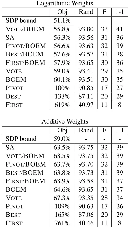
Table 1: Score of the solution with best objective for each solver, averaged over newsgroups training sets, sorted by objective.

metrics (see Meila (2007) for an overview of cluster-ing metrics). The Rand measure counts the number of pairs of points for which the proposed clustering agrees with ground truth. This is the metric which is mathematically closest to the objective. However, since most points are in different clusters, any so-lution with small clusters tends to get a high score. Therefore we also report the more sensitive F-score with respect to the minority (“same cluster”) class. We also report the one-to-one score, which mea-sures accuracy over single points. For this metric, we calculate a maximum-weight matching between proposed clusters and ground-truth clusters, then re-port the overlap between the two.

dis-cussed in Section 4 and the objective value of the singletons clustering (xij = 0, i6=j). On this scale,

lower is better; 0% corresponds to the trivial bound and 100% corresponds to the singletons clustering. It is possible to find values greater than 100%, since some particularly bad clusterings have objectives worse than the singletons clustering. Plainly, how-ever, real clusterings will not have values as low as 0%, since the trivial bound is so unrealistic.

Our results are shown in Table 1. The best re-sults are obtained using logarithmic weights with VOTE followed by BOEM; reasonable results are also found using additive weights, and annealing, VOTE or PIVOT followed by BOEM. On its own, the best greedy scheme is VOTE, but all of them are substantially improved by BOEM. First-link is by far the worst. Our use of the SDP lower bound rather than the trivial lower-bound of 0% reduces the gap between the best clustering and the lower bound by over a factor of ten. It is easy to show that the LP relaxation can obtain a bound of at most 50%6—the SDP beats the LP in both runtime and quality!

We analyze the correlation between objective val-ues and metric valval-ues, averaging Kendall’s tau7over the four datasets (Table 2). Over the entire dataset, correlations are generally good (large and negative), showing that optimizing the objective is indeed a useful way to find good results. We also examine correlations for the solutions with objective values within the top 10%. Here the correlation is much poorer; selecting the solution with the best objective value will not necessarily optimize the metric, al-though the correspondence is slightly better for the log-weights scheme. The correlations do exist, how-ever, and so the solution with the best objective value is typically slightly better than the median.

In Figure 3, we show the distribution of one-to-one scores obtained (for one-to-one specific dataset) by the best solvers. From this diagram, it is clear that log-weights and VOTE/BOEM usually obtain the best scores for this metric, since the median is higher than other solvers’ upper quartile scores. All solvers have quite high variance, with a range of about 2% between quartiles and 4% overall. We omit the

F-6

The solutionxij = 1₂11`w−ij> w

+

ij

´

fori < jis feasible in the LP.

7

The standard Pearson correlation coefficient is less robust to outliers, which causes problems for this data.

BOEMbest/BLbest/Bfirst/Bpivot/BLpivot/BSA L-SAvote/BLvote/B 0.32

0.34 0.36 0.38 0.40 0.42 0.44

Figure 3: Box-and-whisker diagram (outliers as +) for one-to-one scores obtained by the best few solvers on a particular newsgroup dataset. L means using log weights. B means improved with BOEM.

Rand F 1-1 Log-wt -.60 -.73 -.71 Top 10 % -.14 -.22 -.24 Add-wt -.60 -.67 -.65 Top 10 % -.13 -.15 -.14

Table 2: Kendall’s tau correlation between objective and metric values, averaged over newsgroup datasets, for all solutions and top 10% of solutions.

score plot, which is similar, for space reasons.

5.3 Chat Disentanglement

In the disentanglement task, we examine data from a shared discussion group where many conversations are occurring simultaneously. The task is to partition the utterances into a set of conversations. This task differs from newsgroup clustering in that data points (utterances) have an inherent linear order. Ordering is typical in discourse tasks including topic segmen-tation and coreference resolution.

classi-fier made available by Elsner and Charniak (2008);8 this study represents a competitive baseline, al-though more recently Wang and Oard (2009) have improved it. Since this classifier is ineffective at linking utterances more than 129 seconds apart, we treat all decisions for such utterances as abstentions, p = .5. For utterance pairs on which it does make a decision, the classifier has a reported accuracy of 75% with an F-score of 71%.

As in previous work, we run experiments on the 800-utterance test set and average metrics over 6 test annotations. We evaluate using the three metrics re-ported by previous work. Two node-counting met-rics measure global accuracy: one-to-one match as explained above, and Shen’s F (Shen et al., 2006): F = P_i ni

n maxj(F(i, j)). Here i is a gold

con-versation with size ni and j is a proposed

conver-sation with sizenj, sharing nij utterances; F(i, j)

is the harmonic mean of precision (n_nij

j) and recall (nij

ni ). A third metric, the local agreement, counts edgewise agreement for pairs of nearby utterances, where nearby means “within three utterances.”

In this dataset, the SDP is a more moderate im-provement over the trivial lower bound, reducing the gap between the best clustering and best lower bound by a factor of about 3 (Table 3).

Optimization of the objective does not correspond to improvements in the global metrics (Table 3); for instance, the best objectives are attained with FIRST/BOEM, but VOTE/BOEM yields better one-to-one and F scores. Correlation between the ob-jective and these global metrics is extremely weak (Table 5). The local metric is somewhat correlated.

Local search does improve metric results for each particular greedy algorithm. For instance, when BOEM is added to VOTE (with log weights), one-to-one increases from 44% to 46%, local from 72% to 73% and F from 48% to 50%. This represents a moderate improvement on the inference scheme de-scribed in Elsner and Charniak (2008). They use voting with additive weights, but rather than per-forming multiple runs over random permutations, they process utterances in the order they occur. (We experimented with processing in order; the results are unclear, but there is a slight trend toward worse performance, as in this case.) Their results (also

8_{Downloaded fromcs.brown.edu/}

∼melsner

shown in the table) are 41% one-to-one, 73% local and .44% F-score.9 Our improvement on the global metrics (12% relative improvement in one-to-one, 13% in F-score) is modest, but was achieved with better inference on exactly the same input.

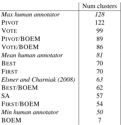
Since the objective function fails to distinguish good solutions from bad ones, we examine the types of solutions found by different methods in the hope of explaining why some perform better than others. In this setting, some methods (notably local search run on its own or from a poor starting point) find far fewer clusters than others (Table 4; log weights not shown but similar to additive). Since the classifier abstains for utterances more than 129 seconds apart, the objective is unaffected if very distant utterances are linked on the basis of little or no evidence; this is presumably how such large clusters form. (This raises the question of whether abstentions should be given weaker links withp < .5. We leave this for future work.) Algorithms which find reasonable numbers of clusters (VOTE, PIVOT, BEST and lo-cal searches based on these) all achieve good metric scores, although there is still no reliable way to find the best solution among this set of methods.

6 Conclusions

It is clear from these results that heuristic methods can provide good correlation clustering solutions on datasets far too large for ILP to scale. The particular solver chosen10has a substantial impact on the qual-ity of results obtained, in terms of external metrics as well as objective value.

For general problems, our recommendation is to use log weights and run VOTE/BOEM. This algo-rithm is fast, achieves good objective values, and yields good metric scores on our datasets. Although objective values are usually only weakly correlated with metrics, our results suggest that slightly bet-ter scores can be obtained by running the algorithm many times and returning the solution with the best objective. This may be worth trying even when the datapoints are inherently ordered, as in chat.

9

The F-score metric is not used in Elsner and Charniak (2008); we compute it ourselves on the result produced by their software.

10_{Our C++ correlation clustering software and SDP} bounding package are available for download from

Log Weights

Obj 1-1 Loc3 Shen F

SDP bound 13.0% - -

-FIRST/BOEM 19.3% 41 74 44 VOTE/BOEM 20.0% 46 73 50

SA 20.3% 42 73 45

BEST/BOEM 21.3% 43 73 47

BOEM 21.5% 22 72 21

PIVOT/BOEM 22.0% 45 72 50

VOTE 26.3% 44 72 48

BEST 37.1% 40 67 44

PIVOT 44.4% 39 66 44

FIRST 58.3% 39 62 41

Additive Weights

Obj 1-1 Loc3 Shen F

SDP bound 16.2% - -

-FIRST/BOEM 21.7% 40 73 44

BOEM 22.3% 22 73 20

BEST/BOEM 22.7% 44 74 49

VOTE/BOEM 23.3% 46 73 50

SA 23.8% 41 72 46

PIVOT/BOEM 24.8% 46 73 50

VOTE 30.5% 44 71 49

EC ’08 - 41 73 44

BEST 42.1% 43 69 47

PIVOT 48.4% 38 67 44

FIRST 69.0% 40 59 41

Table 3: Score of the solution with best objective found by each solver on the chat test dataset, averaged over 6 annotations, sorted by objective.

Whatever algorithm is used to provide an initial solution, we advise the use of local search as a post-process. BOEM always improves both objective and metric values over its starting point.

The objective value is not always sufficient to se-lect a good solution (as in the chat dataset). If pos-sible, experimenters should check statistics like the number of clusters found to make sure they conform roughly to expectations. Algorithms that find far too many or too few clusters, regardless of objec-tive, are unlikely to be useful. This type of problem can be especially dangerous if the pairwise classifier abstains for many pairs of points.

SDP provides much tighter bounds than the trivial bound used in previous work, although how much

Num clusters

Max human annotator 128

PIVOT 122

VOTE 99

PIVOT/BOEM 89

VOTE/BOEM 86

Mean human annotator 81

BEST 70

FIRST 70

Elsner and Charniak (2008) 63

BEST/BOEM 62

SA 57

FIRST/BOEM 54

Min human annotator 50

BOEM 7

Table 4: Average number of clusters found (using addi-tive weights) for chat test data.

1-1 Loc3 Shen F

Log-wt -.40 -.68 -.35 Top 10 % .14 -.15 .15 Add-wt -.31 -.67 -.25 Top 10 % -.07 -.22 .13

Table 5: Kendall’s tau correlation between objective and metric values for the chat test set, for all solutions and top 10% of solutions.

tighter varies with dataset (about 12 times smaller for newsgroups, 3 times for chat). This bound can be used to evaluate the absolute performance of our solvers; the VOTE/BOEM solver whose use we rec-ommend is within about 5% of optimality. Some of this 5% represents the difference between the bound and optimality; the rest is the difference between the optimum and the solution found. If the bound were exactly optimal, we could expect a significant im-provement on our best results, but not a very large one—especially since correlation between objective and metric values grows weaker for the best solu-tions. While it might be useful to investigate more sophisticated local searches in an attempt to close the gap, we do not view this as a priority.

Acknowledgements

References

Nir Ailon, Moses Charikar, and Alantha Newman. 2008. Aggregating inconsistent information: Ranking and clustering. Journal of the ACM, 55(5):Article No. 23. Nikhil Bansal, Avrim Blum, and Shuchi Chawla. 2004.

Correlation clustering. Machine Learning,

56(1-3):89–113.

Regina Barzilay and Mirella Lapata. 2006. Aggregation via set partitioning for natural language generation. In

HLT-NAACL.

Amir Ben-Dor, Ron Shamir, and Zohar Yakhini. 1999. Clustering gene expression patterns. Journal of

Com-putational Biology, 6(3-4):281–297.

Michael Bertolacci and Anthony Wirth. 2007. Are approximation algorithms for consensus clustering worthwhile? In SDM ’07: Procs. 7th SIAM Inter-national Conference on Data Mining.

Moses Charikar, Venkatesan Guruswami, and Anthony Wirth. 2005. Clustering with qualitative information.

J. Comput. Syst. Sci., 71(3):360–383.

William W. Cohen and Jacob Richman. 2002. Learn-ing to match and cluster large high-dimensional data sets for data integration. In KDD ’02, pages 475–480. ACM.

Scott Deerwester, Susan T. Dumais, George W. Furnas, Thomas K. Landauer, and Richard Harshman. 1990. Indexing by latent semantic analysis. Journal of the

American Society for Information Science, 41:391–

407.

Erik D. Demaine, Dotan Emanuel, Amos Fiat, and Nicole Immorlica. 2006. Correlation clustering in general weighted graphs. Theor. Comput. Sci., 361(2):172– 187.

Micha Elsner and Eugene Charniak. 2008. You talk-ing to me? a corpus and algorithm for conversation disentanglement. In Proceedings of ACL-08: HLT, pages 834–842, Columbus, Ohio, June. Association for Computational Linguistics.

Jenny Rose Finkel and Christopher D. Manning. 2008. Enforcing transitivity in coreference resolution. In

Proceedings of ACL-08: HLT, Short Papers, pages 45–

48, Columbus, Ohio, June. Association for Computa-tional Linguistics.

Aristides Gionis, Heikki Mannila, and Panayiotis Tsaparas. 2007. Clustering aggregation. ACM Trans.

on Knowledge Discovery from Data, 1(1):Article 4.

Ioannis Giotis and Venkatesan Guruswami. 2006. Corre-lation clustering with a fixed number of clusters.

The-ory of Computing, 2(1):249–266.

Andrey Goder and Vladimir Filkov. 2008. Consensus clustering algorithms: Comparison and refinement. In

ALENEX ’08: Procs. 10thWorkshop on Algorithm En-ginering and Experiments, pages 109–117. SIAM.

Cristoph Helmberg. 2000. Semidefinite programming for combinatorial optimization. Technical Report ZR-00-34, Konrad-Zuse-Zentrum f¨ur Informationstechnik Berlin.

Cristoph Helmberg, 2009. The ConicBundle Li-brary for Convex Optimization. Ver. 0.2i from http://www-user.tu-chemnitz.de

/_∼helmberg/ConicBundle/.

Thorsten Joachims and John Hopcroft. 2005. Error bounds for correlation clustering. In ICML ’05, pages 385–392, New York, NY, USA. ACM.

Thorsten Joachims. 1997. A probabilistic analysis of the Rocchio algorithm with TFIDF for text categoriza-tion. In International Conference on Machine

Learn-ing (ICML), pages 143–151.

Igor Malioutov and Regina Barzilay. 2006. Minimum cut model for spoken lecture segmentation. In ACL. The Association for Computer Linguistics.

Claire Mathieu and Warren Schudy. 2008. Correlation clustering with noisy input. Unpublished manuscript available from http://www.cs.brown.edu/_∼ws/papers/clustering.pdf. Andrew McCallum and Ben Wellner. 2004.

Condi-tional models of identity uncertainty with application to noun coreference. In Proceedings of the 18th

An-nual Conference on Neural Information Processing Systems (NIPS), pages 905–912. MIT Press.

Marina Meila. 2007. Comparing clusterings–an infor-mation based distance. Journal of Multivariate

Analy-sis, 98(5):873–895, May.

Vincent Ng and Claire Cardie. 2002. Improving machine learning approaches to coreference resolution. In

Pro-ceedings of the 40th Annual Meeting of the Association for Computational Linguistics, pages 104–111.

Dou Shen, Qiang Yang, Jian-Tao Sun, and Zheng Chen. 2006. Thread detection in dynamic text message streams. In SIGIR ’06, pages 35–42, New York, NY, USA. ACM.

Wee Meng Soon, Hwee Tou Ng, and Daniel Chung Yong Lim. 2001. A machine learning approach to corefer-ence resolution of noun phrases. Computational

Lin-guistics, 27(4):521–544.

Lidan Wang and Douglas W. Oard. 2009. Context-based message expansion for disentanglement of interleaved text conversations. In Proceedings of NAACL-09 (to

appear).

Shi Zhong and Joydeep Ghosh. 2003. Model-based clus-tering with soft balancing. In ICDM ’03: Proceedings

of the Third IEEE International Conference on Data Mining, page 459, Washington, DC, USA. IEEE