SHEF-Lite: When Less is More for Translation Quality Estimation
Daniel Beck and Kashif Shah and Trevor Cohn and Lucia Specia
Department of Computer Science University of Sheffield Sheffield, United Kingdom
{debeck1,kashif.shah,t.cohn,l.specia}@sheffield.ac.uk
Abstract
We describe the results of our submissions to the WMT13 Shared Task on Quality Estimation (subtasks 1.1 and 1.3). Our submissions use the framework of Gaus-sian Processes to investigate lightweight approaches for this problem. We focus on two approaches, one based on feature se-lection and another based on active learn-ing. Using only 25 (out of 160) fea-tures, our model resulting from feature selection ranked 1st place in the scoring variant of subtask 1.1 and 3rd place in the ranking variant of the subtask, while the active learning model reached 2nd place in the scoring variant using only
∼25% of the available instances for
train-ing. These results give evidence that Gaussian Processes achieve the state of the art performance as a modelling ap-proach for translation quality estimation, and that carefully selecting features and instances for the problem can further im-prove or at least maintain the same per-formance levels while making the problem less resource-intensive.
1 Introduction
The purpose of machine translation (MT) quality estimation (QE) is to provide a quality prediction for new, unseen machine translated texts, with-out relying on reference translations (Blatz et al., 2004; Specia et al., 2009; Callison-burch et al., 2012). A common use of quality predictions is the decision between post-editing a given machine translated sentence and translating its source from scratch, based on whether its post-editing effort is estimated to be lower than the effort of translating the source sentence.
The WMT13 QE shared task defined a group of tasks related to QE. In this paper, we present
the submissions by the University of Sheffield team. Our models are based on Gaussian Pro-cesses (GP) (Rasmussen and Williams, 2006), a non-parametric probabilistic framework. We ex-plore the application of GP models in two con-texts: 1) improving the prediction performance by applying a feature selection step based on opti-mised hyperparameters and 2) reducing the dataset size (and therefore the annotation effort) by per-forming Active Learning (AL). We submitted en-tries for two of the four proposed tasks.
Task 1.1 focused on predicting HTER scores (Human Translation Error Rate) (Snover et al., 2006) using a dataset composed of 2254 English-Spanish news sentences translated by Moses (Koehn et al., 2007) and post-edited by a profes-sional translator. The evaluation used a blind test set, measuring MAE (Mean Absolute Error) and RMSE (Root Mean Square Error), in the case of the scoring variant, and DeltaAvg and Spearman’s rank correlation in the case of the ranking vari-ant. Our submissions reached 1st (feature selec-tion) and 2nd (active learning) places in the scor-ing variant, the task the models were optimised for, and outperformed the baseline by a large mar-gin in the ranking variant.
The aim of task 1.3 aimed at predicting post-editing time using a dataset composed of 800 English-Spanish news sentences also translated by Moses but post-edited by five expert translators. Evaluation was done based on MAE and RMSE on a blind test set. For this task our models were not able to beat the baseline system, showing that more advanced modelling techniques should have been used for challenging quality annotation types and datasets such as this.
2 Features
In our experiments, we used a set of 160 features which are grouped intoblack box(BB) and glass box(GB) features. They were extracted using the
open source toolkit QuEst1 (Specia et al., 2013).
We briefly describe them here, for a detailed de-scription we refer the reader to the lists available on the QuEst website.
The 112 BB features are based on source and target segments and attempt to quantify the source
complexity, the target fluency and the source-targetadequacy. Examples of them include:
• Word and n-gram based features:
– Number of tokens in source and target segments;
– Language model (LM) probability of source and target segments;
– Percentage of source 1–3-grams ob-served in different frequency quartiles of the source side of the MT training cor-pus;
– Average number of translations per source word in the segment as given by IBM 1 model with probabilities thresh-olded in different ways.
• POS-based features:
– Ratio of percentage of nouns/verbs/etc in the source and target segments;
– Ratio of punctuation symbols in source and target segments;
– Percentage of direct object personal or possessive pronouns incorrectly trans-lated.
• Syntactic features:
– Source and target Probabilistic Context-free Grammar (PCFG) parse log-likelihood;
– Source and target PCFG average confi-dence of all possible parse trees in the parser’s n-best list;
– Difference between the number of PP/NP/VP/ADJP/ADVP/CONJP phrases in the source and target;
• Other features:
– Kullback-Leibler divergence of source and target topic model distributions;
– Jensen-Shannon divergence of source and target topic model distributions;
1http://www.quest.dcs.shef.ac.uk
– Source and target sentence intra-lingual mutual information;
– Source-target sentence inter-lingual mu-tual information;
– Geometric average of target word prob-abilities under a global lexicon model.
The 48 GB features are based on information provided by the Moses decoder, and attempt to in-dicate theconfidenceof the system in producing the translation. They include:
• Features and global score of the SMT model;
• Number of distinct hypotheses in the n-best list;
• 1–3-gram LM probabilities using translations in the n-best to train the LM;
• Average size of the target phrases;
• Relative frequency of the words in the
trans-lation in the n-best list;
• Ratio of SMT model score of the top
transla-tion to the sum of the scores of all hypothesis in the n-best list;
• Average size of hypotheses in the n-best list;
• N-best list density (vocabulary size / average sentence length);
• Fertility of the words in the source sentence
compared to the n-best list in terms of words (vocabulary size / source sentence length);
• Edit distance of the current hypothesis to the centre hypothesis;
• Proportion of pruned search graph nodes;
• Proportion of recombined graph nodes.
3 Model
Gaussian Processes are a Bayesian non-parametric machine learning framework considered the state-of-the-art for regression. They assume the pres-ence of a latent functionf :RF →R, which maps a vectorxfrom feature spaceF to a scalar value.
Formally, this function is drawn from a GP prior:
f(x)∼ GP(0, k(x,x0))
which is parameterized by a mean function (here,
response value is then generated from the function evaluated at the corresponding input,yi=f(xi)+
η, whereη∼ N(0, σn2)is added white-noise. Prediction is formulated as a Bayesian inference under the posterior:
p(y∗|x∗,D) =
Z
f
p(y∗|x∗, f)p(f|D)
where x∗ is a test input, y∗ is the test response value andDis the training set. The predictive pos-terior can be solved analitically, resulting in:
y∗ ∼ N(kT∗(K+σ2nI)−1y,
k(x∗, x∗)−kT∗(K+σ2nI)−1k∗)
where k∗ = [k(x∗,x1)k(x∗,x2). . . k(x∗,xd)]T is the vector of kernel evaluations between the training set and the test input andK is the kernel
matrix over the training inputs.
A nice property of this formulation is that y∗
is actually a probability distribution, encoding the model uncertainty and making it possible to inte-grate it into subsequent processing. In this work, we used the variance values given by the model in an active learning setting, as explained in Section 4.
The kernel function encodes the covariance (similarity) between each input pair. While a vari-ety of kernel functions are available, here we fol-lowed previous work on QE using GP (Cohn and Specia, 2013; Shah et al., 2013) and employed a squared exponential (SE) kernel with automatic relevance determination (ARD):
k(x,x0) =σ2f exp −1 2
F
X
i=1
xi−x0i
li
!
whereF is the number of features, σf2 is the
co-variance magnitude and li > 0 are the feature length scales.
The resulting model hyperparameters (SE vari-anceσ2f, noise varianceσn2and SE length scalesli) were learned from data by maximising the model likelihood. In general, the likelihood function is non-convex and the optimisation procedure may lead to local optima. To avoid poor hyperparam-eter values due to this, we performed a two-step procedure where we first optimise a model with all the SE length scales tied to the same value (which is equivalent to an isotropic model) and we used the resulting values as starting point for the ARD optimisation.
All our models were trained using the GPy2
toolkit, an open source implementation of GPs written in Python.
3.1 Feature Selection
To perform feature selection, we followed the ap-proach used in Shah et al. (2013) and ranked the features according to their learned length scales (from the lowest to the highest). The length scales of a feature can be interpreted as the relevance of such feature for the model. Therefore, the out-come of a GP model using an ARD kernel can be viewed as a list of features ranked by relevance, and this information can be used for feature selec-tion by discarding the lowest ranked (least useful) ones.
For task 1.1, we performed this feature selection over all 160 features mentioned in Section 2. For task 1.3, we used a subset of the 80 most general BB features as in (Shah et al., 2013), for which we had all the necessary resources available for the extraction. We selected the top 25 features for both models, based on empirical results found by Shah et al. (2013) for a number of datasets, and then retrained the GP using only the selected features.
4 Active Learning
Active Learning (AL) is a machine learning paradigm that let the learner decide which data it wants to learn from (Settles, 2010). The main goal of AL is to reduce the size of the dataset while keeping similar model performance (therefore re-ducing annotation costs). In previous work with 17 baseline features, we have shown that with only
∼30% of instances it is possible to achieve 99%
of the full dataset performance in the case of the WMT12 QE dataset (Beck et al., 2013).
To investigate if a reduced dataset can achieve competitive performance in a blind evaluation set-ting, we submitted an entry for both tasks 1.1 and 1.3 composed of models trained on a subset of in-stances selected using AL, and paired with fea-ture selection. Our AL procedure starts with a model trained on a small number of randomly se-lected instances from the training set and then uses this model to query the remaining instances in the training set (our query pool). At every iteration, the model selects the more “informative” instance, asks an oracle for its true label (which in our case is already given in the dataset, and therefore we
only simulate AL) and then adds it to the training set. Our procedure started with 50 instances for task 1.1 and 20 instances for task 1.3, given its re-duced training set size. We optimised the Gaussian Process hyperparameters every 20 new instances, for both tasks.
As a measure of informativeness we used Infor-mation Density (ID) (Settles and Craven, 2008). This measure leverages between the variance among instances and how dense the region (in the feature space) where the instance is located is:
ID(x) =V ar(y|x)× 1
U
U
X
u=1
sim(x,x(u))
!β
The β parameter controls the relative
impor-tance of the density term. In our experiments, we set it to 1, giving equal weights to variance and density. The U term is the number of instances
in the query pool. The variance valuesV ar(y|x) are given by the GP prediction while the similar-ity measuresim(x,x(u)) is defined as the cosine distance between the feature vectors.
In a real annotation setting, it is important to decide when to stop adding new instances to the training set. In this work, we used the confidence method proposed by Vlachos (2008). This is an method that measures the model’s confidence on a held-out non-annotated dataset every time a new instance is added to the training set and stops the AL procedure when this confidence starts to drop. In our experiments, we used the average test set variance as the confidence measure.
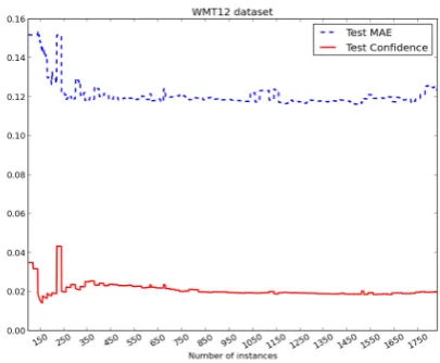
In his work, Vlachos (2008) showed a correla-tion between the confidence and test error, which motivates its use as a stop criterion. To check if this correlation also occurs in our task, we measure the confidence and test set error for task 1.1 using the WMT12 split (1832/422 instances). However, we observed a different behaviour in our experi-ments: Figure 1 shows that the confidence does not raise or drop according to the test error but it stabilisesaround a fixed value at the same point as the test error also stabilises. Therefore, instead of using the confidence dropas a stop criterion, we use the point where the confidence stabilises. In Figure 2 we can observe that the confidence curve for the WMT13 test set stabilises after∼580
[image:4.595.312.515.63.230.2]in-stances. We took that point as our stop criterion and used the first 580 selected instances as the AL dataset.
[image:4.595.313.517.301.468.2]Figure 1: Test error and test confidence curves for HTER prediction (task 1.1) using the WMT12 training and test sets.
Figure 2: Test confidence for HTER prediction (task 1.1) using the official WMT13 training and test sets.
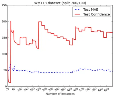
We repeated the experiment with task 1.3, mea-suring the relationship between test confidence and error using a 700/100 instances split (shown on Figure 3). For this task, the curves did not fol-low the same behaviour: the confidence do not seem to stabilise at any point in the AL proce-dure. The same occurred when using the official training and test sets (shown on Figure 4). How-ever, the MAE curve is quite flat, stabilising after about 100 sentences. This may simply be a conse-quence of the fact that our model is too simple for post-editing time prediction. Nevertheless, in or-der to analyse the performance of AL for this task we submitted an entry using the first 100 instances chosen by the AL procedure for training.
re-Task 1.1 - Ranking Task 1.1 - Scoring Task 1.3
DeltaAvg↑ Spearman↑ MAE↓ RMSE↓ MAE↓ RMSE↓
SHEF-Lite-FULL 9.76 0.57 12.42 15.74 55.91 103.11
SHEF-Lite-AL 8.85 0.50 13.02 17.03 64.62 99.09
[image:5.595.90.503.62.134.2]Baseline 8.52 0.46 14.81 18.22 51.93 93.36
[image:5.595.88.285.193.360.2]Table 1: Submission results for tasks 1.1 and 1.3. The bold value shows a winning entry in the shared task.
Figure 3: Test error and test confidence curves for post-editing time prediction (task 1.3) using a 700/100 split on the WMT13 training set.
Figure 4: Test confidence for post-editing time prediction (task 1.3) using the official WMT13 training and test sets.
sult from steps where the hyperparameter optimi-sation got stuck at bad local optima. These de-generated results set the variances (σ2
f,σ2n) to very high values, resulting in a model that considers all data as pure noise. Since this behaviour tends to disappear as more instances are added to the
train-ing set, we believe that increastrain-ing the dataset size helps to tackle this problem. We plan to investi-gate this issue in more depth in future work.
For both AL datasets we repeated the feature se-lection procedure explained in Section 3.1, retrain-ing the models on the selected features.
5 Results
Table 1 shows the results for both tasks. SHEF-Lite-FULL represents GP models trained on the full dataset (relative to each task) with a feature selection step. SHEF-Lite-AL corresponds to the same models trained on datasets obtained from each active learning procedure and followed by feature selection.
For task 1.1, our submission SHEF-Lite-FULL was the winning system in the scoring subtask, and ranked third in the ranking subtask. These results show that GP models achieve the state of the art performance in QE. These are particularly positive results considering that there is room for improve-ment in the feature selection procedure to identify the optimal number of features to be selected. Re-sults for task 1.3 were below the baseline, once again evidencing the fact that the noise model used in our experiments is probably too simple for post-editing time prediction. Post-post-editing time is gener-ally more prone to large variations and noise than HTER, especially when annotations are produced by multiple post-editors. Therefore we believe that kernels that encode more advanced noise models (such as the multi-task kernel used by Cohn and Specia (2013)) should be used for better perfor-mance. Another possible reason for that is the smaller set of features used for this task (black-box features only).
[image:5.595.89.285.439.605.2]an-notation needs. We note however that these results are below those obtained with the full training set, but Figure 1 shows that it is possible to achieve the same or even better results with an AL dataset. Since the curves shown in Figure 1 were obtained using the full feature set, we believe that advanced feature selection strategies can help AL datasets to achieve better results.
6 Conclusions
The results obtained by our submissions confirm the potential of Gaussian Processes to become the state of the art approach for Quality Estimation. Our models were able to achieve the best perfor-mance in predicting HTER. They also offer the ad-vantage of inferring a probability distribution for each prediction. These distributions provide richer information (like variance values) that can be use-ful, for example, in active learning settings.
In the future, we plan to further investigate these models by devising more advanced kernels and feature selection methods. Specifically, we want to employ our feature set in a multi-task kernel set-ting, similar to the one proposed by Cohn and Spe-cia (2013). These kernels have the power to model inter-annotator variance and noise, which can lead to better results in the prediction of post-editing time.
We also plan to pursue better active learning procedures by investigating query methods specif-ically tailored for QE, as well as a better stop cri-teria. Our goal is to be able to reduce the dataset size significantly without hurting the performance of the model. This is specially interesting in the case of QE, since it is a very task-specific problem that may demand a large annotation effort.
Acknowledgments
This work was supported by funding from CNPq/Brazil (No. 237999/2012-9, Daniel Beck) and from the EU FP7-ICT QTLaunchPad project (No. 296347, Kashif Shah and Lucia Specia).
References
Daniel Beck, Lucia Specia, and Trevor Cohn. 2013. Reducing Annotation Effort for Quality Estimation via Active Learning. InProceedings of ACL (to ap-pear).
John Blatz, Erin Fitzgerald, and George Foster. 2004. Confidence estimation for machine translation. In
Proceedings of the 20th Conference on Computa-tional Linguistics, pages 315–321.
Chris Callison-burch, Philipp Koehn, Christof Monz, Matt Post, Radu Soricut, and Lucia Specia. 2012. Findings of the 2012 Workshop on Statistical Ma-chine Translation. InProceedings of 7th Workshop on Statistical Machine Translation.
Trevor Cohn and Lucia Specia. 2013. Modelling Annotator Bias with Multi-task Gaussian Processes: An Application to Machine Translation Quality Es-timation. InProceedings of ACL (to appear).
Philipp Koehn, Hieu Hoang, Alexandra Birch, Chris Callison-Burch, Marcello Federico, Nicola Bertoldi, Brooke Cowan, Wade Shen, Christine Moran, Richard Zens, Chris Dyer, Ondrej Bojar, Alexandra Constantin, and Evan Herbst. 2007. Moses: Open source toolkit for statistical machine translation. In
Proceedings of the 45th Annual Meeting of the ACL on Interactive Poster and Demonstration Sessions, pages 177–180.
Carl Edward Rasmussen and Christopher K. I. Williams. 2006. Gaussian processes for machine learning, volume 1. MIT Press Cambridge.
Burr Settles and Mark Craven. 2008. An analysis of active learning strategies for sequence labeling tasks. InProceedings of the Conference on Empiri-cal Methods in Natural Language Processing, pages 1070–1079.
Burr Settles. 2010. Active learning literature survey. Technical report.
Kashif Shah, Trevor Cohn, and Lucia Specia. 2013. An Investigation on the Effectiveness of Features for Translation Quality Estimation. InProceedings of MT Summit XIV (to appear).
Matthew Snover, Bonnie Dorr, Richard Schwartz, Lin-nea Micciulla, and John Makhoul. 2006. A study of translation edit rate with targeted human annotation. InProceedings of Association for Machine Transla-tion in the Americas.
Lucia Specia, Craig Saunders, Marco Turchi, Zhuoran Wang, and John Shawe-Taylor. 2009. Improving the confidence of machine translation quality esti-mates. InProceedings of MT Summit XII.
Lucia Specia, Kashif Shah, Jos´e G. C. De Souza, and Trevor Cohn. 2013. QuEst - A translation qual-ity estimation framework. In Proceedings of ACL Demo Session (to appear).