Quality estimation for Machine Translation output using linguistic analysis and decoding features

Quality Estimation for Machine Translation output

using linguistic analysis and decoding features

Eleftherios Avramidis

German Research Center for Artificial Intelligence (DFKI) Berlin, Germany

[email protected]

Abstract

We describe a submission to the WMT12 Quality Estimation task, including an exten-sive Machine Learning experimentation. Data were augmented with features from linguis-tic analysis and statislinguis-tical features from the SMT search graph. Several Feature Selec-tion algorithms were employed. The Quality Estimation problem was addressed both as a regression task and as a discretised classifi-cation task, but the latter did not generalise well on the unseen testset. The most success-ful regression methods had an RMSE of 0.86 and were trained with a feature set given by Correlation-based Feature Selection. Indica-tions that RMSE is not always sufficient for measuring performance were observed.

1 Introduction

As Machine Translation (MT) gradually gains a po-sition into production environments, the need for es-timating the quality of its output is increasing. Vari-ous use cases refer to it as input assessment for Hu-man Post-editing, as an extension for Hybrid MT or System Combination, or even a method for improv-ing components of existimprov-ing MT systems.

With the current submission we are trying to address the problem of assigning a quality score to a single MT output per source sentence. Pre-vious work includes regression methods for in-dicating a binary value of correctness (Quirk, 2001; Blatz et al., 2004; Ueffing and Ney, 2007), human-likeness (Gamon et al., 2005) or continu-ous scores (Specia et al., 2009). As we also work with continuous scores, we are making an effort to combine previous feature acquisition sources,

such as language modelling (Raybaud et al., 2009), language fluency checking (Parton et al., 2011), parsing (S´anchez-Martinez, 2011; Avramidis et al., 2011) and decoding statistics (Specia et al., 2009; Avramidis, 2011). The current submission combines such previous observations in a combinatory experi-mentation on feature sets, feature selection methods and Machine Learning (ML) algorithms.

The structure of the submission is as follows: The approach is defined and the methods are described in section 2, including features acquisition, feature selection and learning. Section 3 includes informa-tion about the experiment setup whereas the results are discussed in Section 4.

2 Methods

2.1 Data and basic approach

This contribution has been built based on the data released for the Quality Estimation task of the Workshop on Machine Translation (WMT) 2012 (Callison-Burch et al., 2012). The organizers pro-vided an English-to-Spanish development set and a test set of 1832 and 422 sentences respectively, de-rived from WMT09 and WMT10 datasets. For each source sentence of the development set, participants were offered one translation generated by a state-of-the-art phrase-based SMT system. The quality of each SMT translation was assessed by human evalu-ators, who provided a quality score in the range 1-5. Additionally, statistics and processing information from the execution of the SMT decoding algorithm were given.

The approach presented here is making use of the source sentences, the SMT output and the quality scores in order to follow a typical ML paradigm:

sentence suggestion

. . . los l´ıderes de la Uni´on han descrito comodeducciones pol´ıtico. . . number agreement La articulary ideol´ogicamenteconvencido de asesino de masas . . . transform “y” to “e” Right afterhearingabout it, he described it as a “challenge. . . ” disambiguate -ing

Table 1: Sample suggestions generated by rule-based language checking tools, observed in development data

each source and target sentence of the development set are being analyzed to generate a feature vector. One training sample is formed out of the feature vec-tor and the quality score (i.e. as a class value) of each sentence. A ML algorithm is consequently used to train a model given the training samples. The per-formance of each model is evaluated upon a part of the development set that was kept-out from training.

2.2 Acquiring Features

The features were obtained from two sources: the decoding process and the analysis of the text of the source and the target sentence. The two steps are explained below.

2.2.1 Features from text analysis

The following features were generated with the use of tools for the statistical and/or linguistic analysis of the text. The baseline features included:

• Tokens count: Count of tokens in the source and the translated sentence and their ratio, un-known words and also occurrences of the target word within the translated sentence (averaged for all words in the hypothesis - type/token ra-tio)

• IBM1-model lookup: Average number of translations per source word in the sentence, unweighted or weighted by the inverse fre-quency of each word in the source corpus

• Language modeling: Language model proba-bility of the source and translated sentence

• Corpus lookup: percentage of unigrams / bi-grams / tribi-grams in quartiles 1 and 4 of fre-quency (lower and higher frefre-quency words) in a corpus of the source language

Additionally, the following linguistically motivated features were also included:

• Parsing: PCFG Parse (Petrov et al., 2006) log-likelihood, size of n-best tree list, confidence for the best parse, average confidence of all parse trees. Ratios of the mentioned target fea-tures to the corresponding source feafea-tures.

• Shallow grammatical match: The number of occurences of particular node tags on both the source and the target was counted on the PCFG parses. Additionally, the ratio of the occurences of each tag in the target sentence by the corresponding occurences on the source sentence.

• Language quality check: Source and target sentences were subject to automatic rule-based language quality checking, providing a wide range of quality suggestions concerningstyle,

grammarandterminology, summed up in an overall quality score. The process employed 786 rules for English and 70 rules for Spanish. We counted the occurences of every rule match in each sentence and the number of characters it affected. Sample rule suggestions can be seen in Table 1.

2.2.2 Features from the decoding process

The organisers provided a verbose output of the de-coding process, including probabilistic scores from all steps of the execution of the translation search. We added the scores appearing once per sentence (i.e. referring to the best hypothesis), whereas for the ones being modified over the generation graph, their average (avg), variance (var) and standard de-viation (std) was calculated. These features are:

• the log of the phrase translation probability (pC) and the phrase future cost estimate (c)

• the score component vector including the dis-tortion scores (d1...7), word penalty, translation

Experience has shown difficulties in including hun-dreds of features into training a statistical model. Several algorithms (such as Na¨ıve Bayes) require statistically-independent features. For others, a search space of hundreds of features may impose increased computational complexity, which is often unsustainable in the time and resources allocated. In these cases we therefore applied several common Feature Selectionapproaches, in order to reduce the available features to an affordable number.

We used the Feature Selection algorithms of Re-lieff (Kononenko, 1994), Information Gain and Gain Ratio (Kullback and Leibler, 1951), and Correlation-based Feature Selection (Hall, 2000). The latter is known for producing feature sets highly correlated with the class, yet uncorrelated with each other; selection was done in two variations, greedy stepwiseandbest first.

The data were discretised according to the algo-rithm requirements and features were scored in a 10-fold cross-validation.

2.4 Machine Learning

We tried to approach the issue with two distinct modelling approaches,classificationandregression.

2.4.1 Classification algorithms

In an effort to interpret Quality Estimation as a classification problem, we expect to build models that are able to assign a discrete value, as a mea-sure of sentence quality. This bears some relation to the way the quality scores were generated; humans were asked to provide an (integer) quality score in the range 1-5. In our case, we try to build classifiers that do the same, but are also able to assign values with smaller intervals. For this purpose, we set up 4 sub-experiments, where the class value in our data was rounded up to intervals of 0.25, 0.5, 0.7 and 1.0 respectively.

In this part of the experiment we used theNa¨ıve Bayes,k-nearest-neighbours(kNN),Support Vector Machines(SVM) andTree classificationalgorithms. Na¨ıve Bayes’ probabilities for our continuous fea-tures were estimated withlocally weighted linear re-gression(Cleveland, 1979).

Regression algorithms produce a model for di-rectly predicting a quality score with continu-ous values. Experimentation here included Par-tial Least Squares Regression (Stone and Brooks, 1990), Multivariate Adaptive Regression Splines – MARS (Friedman, 1991), Lasso (Tibshirani, 1994) andLinear Regression.

3 Experiment and Results

3.1 Implementation

PCFG parsing features were generated on the out-put of the Berkeley Parser (Petrov and Klein, 2007), trained over an English and a Spanish tree-bank (Mariona Taul´e and Recasens, 2008). N-gram features have been generated with the SRILM toolkit (Stolcke, 2002). TheAcrolinx IQ1was used to parse the source side, whereas theLanguage Tool2 was applied on both sides.

The feature selection and learning algorithms were implemented with the Orange (Demˇsar et al., 2004) and Weka (Hall et al., 2009) toolkits.

3.2 Experiment structure

The methods explained in the previous section pro-vide a wide range of experiment parameters. Con-sequently, we tried to extensively test all the possi-ble parameter combinations. The development data were separated in two sets, one “training” set and one “keep-out” set, used to test the predictions. In order to give learners better coverage over the data, the development set was split in two ways (70% training - 30% test and 90% training - 10% test), so that all experiments get performed under both set-tings. The scores of these two were averaged3.

3.3 Results

The small size of the dataset allowed for fast train-ing and testtrain-ing of the discrete classification problem, where we could execute 370 experiments. The re-gression problem was considerably slower, as only 36 experiments concluded in time.

1

http://www.acrolinx.com (proprietary)

2

http://languagetool.org (open-source)

3_{Given the disparity of the test sizes, it would have in}

5-fold avg 70-30%, 90-10% folds algorithm feat. set discr. CA AUC RMSE MAE interval Tree #17, #20 0.25 15.40 54.10 0.84 0.67 1.5 5.0 Tree #23 0.25 14.60 53.50 0.85 0.68 2.0 5.0 Tree #12 0.25 13.90 52.00 0.86 0.69 1.8 5.0

Tree #4 0.25 14.50 53.70 0.86 0.69 2.0 5.0

SVM #16 0.25 16.00 60.40 0.86 0.69 3.2 3.2

kNN #22 0.25 12.30 55.50 1.00 0.78 2.0 5.0

Tree #21 0.50 22.70 54.60 0.87 0.69 2.0 5.0

SVM #19 0.50 22.40 60.20 0.91 0.73 2.8 5.0

kNN #12 0.50 20.00 54.70 0.98 0.78 2.2 5.0

Naive #6 0.50 21.20 59.40 0.99 0.76 1.2 5.0

Tree #9 0.70 32.70 53.30 0.89 0.71 3.5 4.9

kNN #12 0.70 28.20 56.10 0.93 0.73 2.5 4.9

SVM #18 0.70 30.90 55.60 0.97 0.77 3.5 4.2

Tree #22 1.00 40.30 55.70 0.90 0.71 2.0 5.0

kNN #22 1.00 40.90 59.10 0.96 0.76 2.5 5.0

Naive #23 1.00 41.00 65.50 1.02 0.78 1.2 5.0

SVM #6 1.00 36.60 51.10 1.02 0.84 3.0 4.0

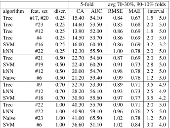
Table 2: Indicative discretised classification results, sorted by best performance and discretisation interval. Classifica-tion Accuracy (AC), Area Under Curve (AUC), Root Mean Square Error (RMSE) and Mean Average Error (MAE), Largest Error Percentage (LEP) and Smallest Error Percentage (SEP)

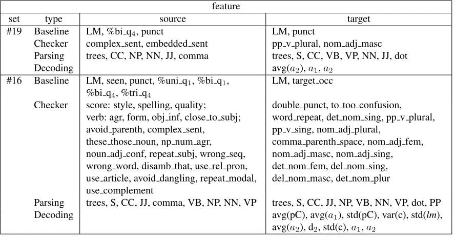
Feature generation resulted (described in Section 2.2) into 266 features, while 90 of them derived from language checking. Feature selection suggested sev-eral feature sets containing between 30 and 80 fea-tures. We ended up defining 22 feature sets, includ-ing the full feature set, the baseline feature set and a couple of manually selected feature sets. Unfor-tunately, due to size restrictions, not all features can be listed; though, indicative feature sets are listed in Table 5.

The most important results of the classification approachcan be seen in Table 2 and the results of theregression approachin Tables 3 (development set) and 4 (shared task test set).

4 Discussion

4.1 Machine Learning Conclusions

Discrete classifiers(section 2.4.1) do not yield en-couraging accuracy, as acceptable levels of accu-racies appear only with a discretisation interval of 1.00, which though cannot be accepted due to its high Root Mean Square Error (RMSE). On the de-velopment keep-out set, the discretised Tree

classi-fier seemingly outperforms all other methods (in-cluding the regression learners), since it yields a RMSE of 0.84, given several different feature vec-tors. Unfortunately, when applied to the final un-known test data, these classifiers performed obvi-ously bad, providing the same single value for all sentences. We could attribute this to overfitting vs. sparse data and consider how we can handle this bet-ter in further work.

Another remarkable observation was the incapa-bility of the RMSE to objectively show the qual-ity of the model, in situations where the predicted values are very close or equal to the average of all real values. A Support Vector Machine with RMSE = 0.86 ranked 3rd among the classifiers, al-though it “cheated” by producing only the average value: 3.25. This leads to the conclusion that the selection of the best algorithm is not just dictated by the lowest RMSE, but it should consider several other indications such as the standard deviation.

We therefore resort to the regression learners

algorithm f. set RMSE MAE interval

PLS #19 0.86 0.69 2.5 4.3

Lasso #19 0.86 0.68 2.7 4.4 Linear #19 0.86 0.68 2.6 4.5

MARS #19 0.86 0.68 2.6 4.7

PLS #18 0.86 0.69 2.7 4.4

Linear #18 0.86 0.69 2.8 4.4 Lasso #18 0.86 0.69 2.8 4.4

MARS #16 0.87 0.69 2.4 4.6

MARS #18 0.86 0.69 2.4 4.5

MARS #4 0.86 0.69 3.4 4.5

PLS #16 0.87 0.70 2.1 4.8

PLS #4 0.87 0.70 2.1 5.4

Linear #4 0.88 0.70 2.4 4.8 Linear #16 0.88 0.70 1.4 4.9

Lasso #4 0.88 0.70 1.9 5.3

MARS #2 0.90 0.72 3.0 4.5

Lasso #16 0.90 0.71 2.7 4.5 Linear #2 0.90 0.72 3.0 4.0

Lasso #2 0.90 0.72 3.0 4.0

PLS #2 0.90 0.73 3.0 3.9

Tree #21 1.08 0.86 1.5 5.0

Tree #19 1.19 0.96 1.6 5.0

Tree #16 1.23 0.98 1.6 5.0

Tree #18 1.25 0.98 1.4 5.0

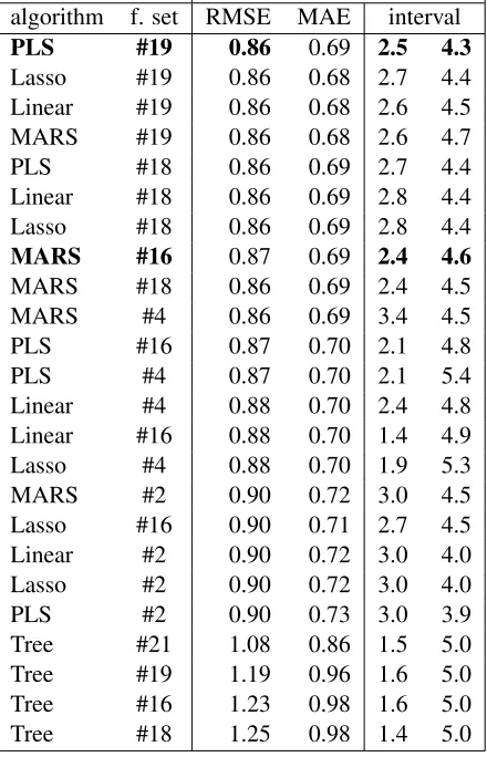
Table 3: Regression results. Root Mean Square Error (RMSE) and Mean Average Error (MAE), Largest Error Percentage (LEP) and Smallest Error Percentage (SEP). Bold face indicates submitted sets

regression algorithms have comparable performance given the same features.

The best-performing feature set (#19) which was chosen as the first submission (DFKI cfs-plsreg) trained with PLS regression, contains features in-dicated by Correlation-based Feature Selection, run withbestfirston a 10-fold cross-validation. We used the features which were selected on the 100% or 90% of the folds. An equally best-performing ture set (#18) has resulted from exactly the same fea-ture selection execution, but contains only feafea-tures which were selected in all folds.

The second submission (DFKI grcfs-mars) was chosen to differentiate both the feature set and the learning method, with respect to a decent interval. Feature set #16 is the result of the Correlation-based

MARS #16 grcfs–mars 0.98 0.82 PLS #19 cfs-plsreg 0.99 0.82

Table 4: Results of the submitted methods on the official testset

Feature Selection, run in a greedy-stepwise mode. The regression was trained with MARS.

The baseline feature set (#2) performed worse. Noticeable was the RMSE of the feature set #4, with features selected based on theirGain Ratio, but we did not submit this due to its very narrow interval.

4.2 Feature conclusions

The best performing feature set gives interesting hints on what worked as a best indication of trans-lation quality. We would try to summarize them as follows:

• The language checking of the source sen-tence detectedcomplexorembedded sentences, which are often not handled properly by SMT due to their complicated structure.

• The language checking of the target sentence detected several agreement issues.

• Parsing provided of source and target count of verbs, nouns, adjectives and secondary sen-tences; with the assumption that translations are relatively isomorphic, the loss of a verb or a noun or the inability to properly handle a sec-ondary sentence, would mean a considerably bad translation outcome. The number of parse trees generated for each sentence can be an in-dication of ambiguity.

• Punctuation (dots, commas) often indicates a complex sentence structure.

• The most useful decoding features were the in-verse phrase translation probability (a₁), the in-verse lexical weighting (a2), the phrase

feature

set type source target

#19 Baseline LM, %bi q4, punct LM, punct

Checker complex sent, embedded sent pp v plural, nom adj masc Parsing trees, CC, NP, NN, JJ, comma trees, S, CC, VB, VP, NN, JJ, dot

Decoding avg(a2),a1,a2

#16 Baseline LM, seen, punct, %uni q1, %bi q1,

%bi q4, %tri q4

LM, target occ

Checker score: style, spelling, quality; verb: agr, form, obj inf, close to subj; avoid parenth, complex sent,

these those noun, np num agr, noun adj conf, repeat subj, wrong seq, wrong word, disamb that, use rel pron, use article, avoid dangling, repeat modal, use complement

double punct, to too confusion, word repeat, det nom sing, pp v plural, pp v sing, nom adj plural,

comma parenth space, nom adj fem, nom adj masc, nom adj sing, det nom fem, del nom sing, del nom masc, det nom plur

Parsing trees, S, CC, JJ, comma, VB, NP, NN, VP trees, S, CC, JJ, NP, VB, NN, VP, dot, PP Decoding avg(pC), avg(a1), std(pC), var(c), std(lm),

avg(a2), d2, std(c),a1,a2

Table 5: Indicative feature sets for the most successful quality estimation models. Features explained at section 2.2

Acknowledgments

This work has been developed within the TaraX ˝U project financed by TSB Technologiestiftung Berlin – Zukunftsfonds Berlin, co-financed by the Euro-pean Union – EuroEuro-pean fund for regional develop-ment. Many thanks to Lukas Poustka for technical help on feature acquisition, to Melanie Siegel for the proprietary language checking tool, and to the re-viewers for the useful comments.

References

Eleftherios Avramidis, Maja Popovic, David Vilar, Aljoscha Burchardt, and Maja Popovi´c. 2011. Evalu-ate with Confidence Estimation : Machine ranking of translation outputs using grammatical features. Pro-ceedings of the Sixth Workshop on Statistical Machine Translation, pages 65–70, July.

Eleftherios Avramidis. 2011. DFKI System Combina-tion with Sentence Ranking at ML4HMT-2011. In

Proceedings of the International Workshop on Using Linguistic Information for Hybrid Machine Transla-tion (LIHMT 2011) and of the Shared Task on Applying Machine Learning Techniques to Optimising the Di-vision of Labour in Hybrid Machine Translation (M. Sha. Center for Language and Speech Technologies and Applications (TALP), Technical University of Cat-alonia.

John Blatz, Erin Fitzgerald, George Foster, Simona Gan-drabur, Cyril Goutte, Alex Kulesza, Alberto Sanchis, and Nicola Ueffing. 2004. Confidence estimation for machine translation. In Proceedings of the 20th in-ternational conference on Computational Linguistics, COLING ’04, Stroudsburg, PA, USA. Association for Computational Linguistics.

Chris Callison-Burch, Philipp Koehn, Christof Monz, Matt Post, Radu Soricut, and Lucia Specia. 2012. Findings of the 2012 workshop on statistical machine translation. InProceedings of the Seventh Workshop on Statistical Machine Translation, Montreal, Canada, June. Association for Computational Linguistics. William S Cleveland. 1979. Robust locally weighted

regression and smoothing scatterplots. Journal of the American statistical association, 74(368):829–836. Janez Demˇsar, Blaz Zupan, Gregor Leban, and Tomaz

Curk. 2004. Orange: From Experimental Machine Learning to Interactive Data Mining. InPrinciples of Data Mining and Knowledge Discovery, pages 537– 539.

Jerome H. Friedman. 1991. Multivariate Adaptive Re-gression Splines.The Annals of Statistics, 19(1):1–67, March.

Michael Gamon, Anthony Aue, and Martine Smets. 2005. Sentence-level MT evaluation without reference translations : Beyond language modeling. Language, (2001):103–111.

SIGKDD Explorations, 11(1):10–18.

Mark A Hall. 2000. Correlation-based Feature Selec-tion for Discrete and Numeric Class Machine Learn-ing. In Pat Langley, editor, Proceedings of 17th In-ternational Conference on Machine Learning, pages 359–366. Morgan Kaufmann Publishers Inc.

Igor Kononenko. 1994. Estimating attributes: anal-ysis and extensions of RELIEF. In Proceedings of the European conference on machine learning on Ma-chine Learning, pages 171–182, Secaucus, NJ, USA. Springer-Verlag New York, Inc.

S Kullback and R A Leibler. 1951. On information and sufficiency. Annals of Mathematical Statistics, 22:49– 86.

M Ant`onia Mart´ı Mariona Taul´e and Marta Recasens. 2008. AnCora: Multilevel Annotated Corpora for Catalan and Spanish. InProceedings of the Sixth In-ternational Conference on Language Resources and Evaluation (LREC’08), Marrakech, Morocco, May. European Language Resources Association (ELRA). Kristen Parton, Joel Tetreault, Nitin Madnani, and Martin

Chodorow. 2011. E-rating Machine Translation. In

Proceedings of the Sixth Workshop on Statistical Ma-chine Translation, pages 108–115, Edinburgh, Scot-land, July. Association for Computational Linguistics. Slav Petrov and Dan Klein. 2007. Improved inference

for unlexicalized parsing. InIn HLT-NAACL 07. Slav Petrov, Leon Barrett, Romain Thibaux, and Dan

Klein. 2006. Learning Accurate, Compact, and Inter-pretable Tree Annotation. InProceedings of the 21st International Conference on Computational Linguis-tics and 44th Annual Meeting of the Association for Computational Linguistics, pages 433–440, Sydney, Australia, July. Association for Computational Lin-guistics.

Christopher B Quirk. 2001. Training a Sentence-Level Machine Translation Confidence Measure. Evalua-tion, pages 825–828.

Sylvain Raybaud, Caroline Lavecchia, David Langlois, and Kamel Sma¨ıli. 2009. New Confidence Measures for Statistical Machine Translation.Proceedings of the International Conference on Agents, pages 394–401. Felipe S´anchez-Martinez. 2011. Choosing the best

ma-chine translation system to translate a sentence by us-ing only source-language information. In Mikel L For-cada, Heidi Depraetere, and Vincent Vandeghinste, ed-itors, Proceedings of the 15th Annual Conference of the European Associtation for Machine Translation, number May, pages 97–104, Leuve, Belgium. Euro-pean Association for Machine Translation.

Lucia Specia, M. Turchi, N. Cancedda, M. Dymetman, and N. Cristianini. 2009. Estimating the Sentence-Level Quality of Machine Translation Systems. In

Machine Translation (EAMT-2009), pages pp. 28–35, Barcelona, Spain.

Andreas Stolcke. 2002. SRILM – An Extensible Lan-guage Modeling Toolkit. InProceedings of the Sev-enth International Conference on Spoken Language Processing, pages 901–904. ISCA, September. M Stone and R J Brooks. 1990. Continuum

regres-sion: cross-validated sequentially constructed predic-tion embracing ordinary least squares, partial least squares and principal components regression.Journal of the Royal Statistical Society Series B Methodologi-cal, 52(2):237–269.

R Tibshirani. 1994. Regression shrinkage and selection via the lasso.

Nicola Ueffing and Hermann Ney. 2007. Word-Level Confidence Estimation for Machine Translation.