Environmental Quality and Economic Growth: A Panel Analysis of the "U" in Kuznets

Munich Personal RePEc Archive

Environmental Quality and Economic

Growth: A Panel Analysis of the "U" in

Kuznets

F. Akpan, Usenobong and E. Abang, Dominic

Department of Economics,University of Uyo, Uyo, Nigeria,

Department of Economics,University of Uyo, Uyo, Nigeria

13 February 2014

Online at

https://mpra.ub.uni-muenchen.de/54461/

1

Environmental Quality and Economic Growth: A Panel Analysis of

the “U” in Kuznets

Usenobong F. Akpan

[email protected]

+234 803 413 0046

&

Dominic E. Abang

_{[email protected]} +234 803 510 3380

Department of Economics,

University of Uyo, Uyo

Nigeria

Abstract

The primary motivation behind this study was to search for evidence of the link between environmental quality and economic growth so as to answer the relevant question of whether economic growth alone could serve as a long-run solution to environmental damage as implied by EKC hypothesis. Here we analyze the relationship using a panel of 47 countries over the period 1970 -2008. Using Random-effect estimation and two-stage least square, our results leads to the following conclusions: relying on a quadratic model can easily mislead researchers to ratify the existence of EKC; the EKC hypothesis ceased to hold whenever an alternative functional form (cubic) is employed. At best, the relationship between economic growth and environmental quality is shown to be typified by an N-shaped curve. The paper maintained that simply waiting for an automatic arrival of a delinking point for environmental damage given long-run growth will not be a feasible solution to environmental quality. A number of feasible policy menu and critical questions to guide selection of the best instrument capable of bringing about a downturn in environmental damage have been suggested in the paper.

Key-words: Economic growth, EKC hypothesis, Environmental quality, delinking

2

1. Introduction

The issue of environmental degradation constitutes one of the greatest concerns for policymakers

especially in the less developed economies. Among other sources, the pollution problems

associated with energy production and consumption has continued to attract global attention. Yet

energy use is vital to economic growth of any nation. This apparent goal conflict poses serious

policy dilemma: reducing environmental degradation or pollution may require reductions in the

rate of economic growth. The solution to this problem seemed to have been found in the 1990s

when some scholars (e.g. Grossman and Krueger, 1991; Shafik and Bandypadhyay, 1992;

Panayotou, 1993) pointed out the existence of an inverted U-shaped relationship between

environmental degradation and economic growth; a relationship which was latter coined by

Panayotou (1993) as Environmental Kuznets Curve (EKC) because of its resemblance to Simon

Kuznet’s income distribution hypothesis. The EKC simply hypothesizes that pollution will first

increase with the level of GDP per capita, reach a maximum and then decrease at higher levels of

income. The policy implications of such findings are clear: economic growth is compatible with

environmental improvements in the long-run as countries could eventually “grow themselves”

out of their environmental problems (Akpan and Chuku, 2011). Stated differently, if EKC

hypothesis holds, then policies that promote economic growth can be pursued with little or no

regard for the corresponding consequences on the environment. In fact, in one of the earliest

studies, Berkerman (1992) strongly submits that:

“…there is clear evidence that, although economic growth usually leads to environmental deterioration in the early stages of the process, in the end the best – and probably the only – way to attain a decent environment in most countries is to become rich”

At the theoretical level, several intuitions have been put forward to justify the existence

of an inverted U-shaped path for environmental damage in the long term. Usually, these

arguments relates to (i) the expected structural changes in the composition of economic output as

a nation develops, (ii) changing technology and input mix (iii)increased environmental

awareness and willingness to pay for cleaner environment at higher income levels and (iv)

development of stronger institutions and capacity to implement environmental laws at higher

3

More succinctly, channels through which an inverted U-shaped path is expected to

emerge for environmental quality and at higher levels of income per capita could be grouped into

three: (i) the scale effect (ii) composition effect (iii) and the technique effect (Grossman and

Krueger, 1991; Stern, 2004; Akpan and Chuku, 2011). It is argued that economic growth will

initially aggravates environmental quality through the scale effect as production is increased at a given factor-input ratio, out-put mix and technology. However, as the structure of the economy

changes (i.e. the output mix changes) from agriculture to more resource intensive manufacturing

industries, pollution increases with growth. At the later stage of development, environmental

quality is expected to improve as the structure of the economy moves towards service and light

manufacturing industries which are supposed to generate lower emissions per unit of output. This

is the composition effect. The technique effect captures the expected improvements in productivity and adaptation of cleaner technologies leading to improvement in environmental

quality. A variant of the technique effect is the input-mix effect which simply underscores the possibility of substituting environmentally harmful inputs by less harmful inputs. An example

includes substituting natural gas for coal.

Based on these arguments, one could have expected pollution to increase in less

developed countries and reduce in more developed nations. But there is nothing automatic that

these expectations would hold. On the one hand, a richer country is likely to use more resources,

demand more energy and produce more waste and pollution than poor countries. On the other

hand and in contrast to poor countries, richer countries may have higher capacity to invest in

renewable energy infrastructure, developed and install state-of-the-art pollution control

equipment and implement effective environmental policies.

Clearly, it is important to understand the nature of the relationship between

environmental degradation and economic growth before advocating the use of EKC as a policy

guide in solving environmental problems. Indeed, if EKC is empirically verified as true, it will

simply imply that environmental damage is an inescapable consequence of growth and therefore

structurally determined. This being the case, any attempt to overcome such damage at the early

stage of development, might be seen as a futile exercise. Thus, given scare economic resources,

the extent to which policy makers ought to allocate available resources in designing and

4

to which the driving forces underlying the EKC are susceptible to such policies (Munasinghe,

1999).

Given the importance of the presumed EKC for economic growth and environmental

sustainability, a large span of research on the existence of EKC have emerged but with mixed

empirical support. For instance, apart from those which have confirmed the existence of EKC

(e.g. Heil and Selden, 2001; Holtz-Eakin and Selden, 1995; Berkerman, 1992; Grossman and

Krueger, 1991; Panayotou, 1993), there are a plethora of others who have found no such

evidence (e.g. Akpan and Chuku, 2011; Friedl and Getzner, 2003; He and Richard, 2010;

Caviglia-Harris, Chambers and Kahn, 2009).

More so, results of studies that have made claim for the existence of EKC have been

disputed and questioned on several fronts. Some of such issues include that of omitted variable

bias, simultaneity bias, and aggregation problem. Stern, et al (1996) has also criticized the tradition of including only high income countries in a given sample by some studies. Such

inclusion ignores different trade patterns and the fact that high-income countries have higher

emission reduction possibilities by outsourcing polluting industries to other countries through

trade specialization or developing strong institutions to implement stringent environmental laws.

On another front, the empirical robustness of the EKC relation remains an open issue (Grossman

and Krueger, 1995). Most often, the reduced form equations in which environmental outcomes

are related to economic growth of the individual countries and to other economic measures often

ignore the feedback from environmental damage to economic activities. If the environmental

damage is sufficiently strong, it is likely that economic activities will be negatively affected and

therefore, ignoring this possibility may not provide a correct picture.

This paper makes robust attempt in addressing the above research gaps. First, we analyze

the relationship using a panel of 47 countries over the period 1970 -2008. For comparative

purpose, apart from pooled results where all the countries are lumped together, we further divide

the sample into high income and low income countries. Second, we make an attempt to resolve

the simultaneity problem by using the two-staged least square (2SLS) estimation technique to

correct for the feedback effect. Third, we test for the validity and consistency of EKC hypothesis

using two functional forms (quadratic and cubic) and controlled for other key variables that are

5

trade and population growth). Based on the empirical evidence, we draw up key policy

implications for environmentally sustainable growth.

2. Methodology

2.1 Model and Data

Traditionally, the analysis of the relationship between some measure of environmental quality

(EQ) and real income per capita (RGDPpc) usually takes the following polynomial approximation in the literature:

= + + + + ; ~ . . . (0, ) (1)

Where and capture country-specific and period specific effects respectively, and is the

stochastic error term assumed to be normally distributed. From the above specification and given

the statistical significance of the income terms, the EKC hypothesis is confirmed to exist if

> 0 and < 0 and the turning point income at which per capita income is at their maximum

level is easily derived as:

( ) ! = "# $−_{2 ' (2)}

However, there are at least two critical specification issues arising from Eq. (1). First, such

specification does not allowed for testing other possible functional forms of the environmental

quality-economic growth relations. Second, estimating Eq. (1) may lead to bias and inconsistent

inferences and parameter estimation owing to omitted variable bias. Specifically, Eq. (1) would

be guilty of specification bias if indeed the true relation between the two variables is cubic rather

than quadratic. To this end, we let the general model to take the following two forms:

= + + ()) * + ($ + ' + ,$ - ' + . / 0

+ 1 + + (3)

= + + ( (+ ,)) * + .$ + '

6

Where FFEC is fossil fuel energy consumption, X/GDP and M/GDP respectively represent the ratio of exports of goods and services to domestic production and the ratio of imports of goods

and services to domestic output, as used in Agras and Chapman (1999). POPg stands for population growth while EP is energy price1. We use per capita CO2 emissions as a proxy for

environmental quality (EQ).

Given their statistical significance, the relationship between income per capita and

environmental quality can be assessed through the signs of the associated beta ( ) coefficients.

For Eq. (3), EKC is confirmed if > 0 and < 0, but if > 0 and = 0, then a

monotonically increasing relationship would be depicted. In the case of Eq. (4), EKC would

equally be indicated provided > 0, < 0 and ₍ = 0. If this holds, then Eq. (2) reduces to

augmenting Eq. (1) with only the control variables. There are other possibilities: > 0, < 0

and ₍ > 0 will reveals a cubic polynomial, representing an N-shaped relationship; > 0, and

= ( = 0 will imply a monotonically increasing relationship; < 0, and = ( = 0 will indicate a monotonically decreasing relationship.

There are clear justifications for the inclusion of control variables in the models. For

instance, fossil fuel energy consumption (FFEC) remains the chief culprit for global carbon dioxide (CO2) emissions, accounting for about 80% of total greenhouse emissions (Akpan &

Akpan, 2012). A priori therefore, this variable is expected to be positive in its coefficient. The

inclusion of the trade variables (X/GDP and M/GDP) allow us to test for the effect of trade on the environment. Theoretically, following the pollution heaven hypothesis, it is argued that pollution-intensive or “dirty” industries would be “displaced” to less developed countries

following the enforcement of strict environmental control laws in the more developed countries

(Akpan & Chuku, 2011). Thus while we expect these variables to have negative relationship with

environmental quality in high income countries, we expect the variables to have direct

relationship with pollution in the case of low income countries.

The possible effect of population on environmental quality is well documented in the

literature. Higher population increases the demand for materials, energy and natural resources

which in turn generates some negative environmental externalities. Thus, the expectation is that

1

7

the pressure of higher population would contribute positively to environmental degradation. The

effect of energy prices in environmental pollution or carbon emission is very revealing. A rise in

energy prices may generates changes in the rate of energy use as well as changes in the structure

of capital and therefore emissions. For instance, consumers may drive less and try to conserve

energy in the home by turning down thermostats. In the long-term, consumers may equally prefer

more fuel efficient cars and make investments in insulation for their homes. In turn, lower energy

prices encourage more fossil fuel consumption which drives environmental pollution. Thus we

expect a negative relationship between energy price (EP) and environmental damage.

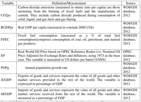
The sources of our data and its construction are shown in Table AI (at the appendix).

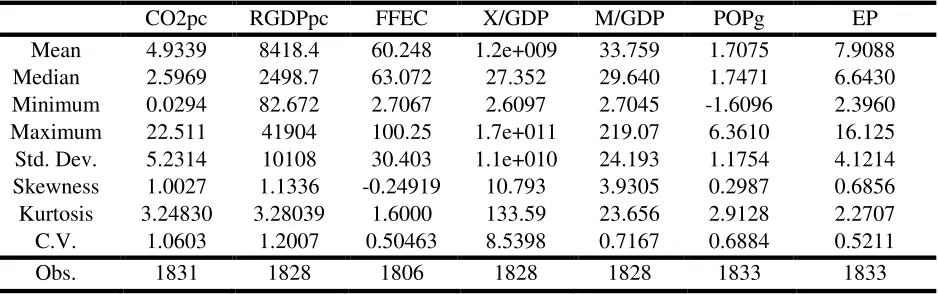
Further, Table A2 (at the appendix) displays the summary statistics of the variables. A close

examination of these descriptive statistics reveals that for most of the variables, the normally

assumption cannot be rejected. In Table A3 (still at the appendix), the correlation matrix of the

variables are presented. Of interest to note is the high and positive correlation (76.2%) between

environmental damage and income per capita as well as with fossil fuel consumption (67.0%). In

addition and as expected, energy price relates negatively with environmental quality (although

the strength of such association is shown to be weak). As a preliminary exercise, we fit a

quadratic curve to a scatter plot of environmental damage and income per capita. This

preliminary result (as shown in Fig. A1, at the appendix) did not present much convincing

evidence for the existence of an inverted U-shaped curve.

2.2 Econometric Procedure

2.2.1 Panel Unit Root and Cointegration Tests

To ensure reliable results, we first examine the stationarity properties of our data set. In

this wise, we consider five sets of panel unit root tests. These include Levin, et al (2002), Breitung (2002), and Im, et al. (2003) tests as well as the ADF Fisher Chi-square test (Dickey and Fuller, 1979) and Phillips-Perron (PP) Fisher Chi-square (Phillips and Perron, 1988). These

constitute a mix of first and second generations panel unit root tests respectively designed to

handle cross-sectionally independent panels and cross-sectional correlation of one form or the

8

and Phillips-Perron (PP) Fisher Chi-square tests assume the presence of individual unit root

processes as their null hypotheses (Akpan and Ekong, 2013).

Specifically, for a brief exposition, the Im, et al. (2003) panel unit root test allows for heterogeneous autoregressive coefficients. It averages the augmented Dickey-Fuller (ADF) unit

root tests of the respective variables while allowing for different orders of serial correlation, = ∑98;: 78 <8+ = , in the following:

> = ? > < + @ 78 9:

8;

<8 + A + + = (5)

Where i = 1,…, N for each country in the panel; t = 1,…, T refers to the time period;+ represents the fixed effects or individual time trend in the model; ? are the autoregressive

coefficients; represents the number of lags in the ADF regression; and are the error terms.

If ? < 1, > is considered weakly trend stationary whereas if ? = 1, then > contains unit

root. The null hypothesis is that each of the series in the panel contains a unit root, while the

alternative is that at least one of the individual series in the panel is stationary.

On the other hand, the ADF Fisher Chi-square test combines the p-values of the test

statistic for a unit root in each residual cross-sectional unit. The test is non-parametric and has a

chi-square distribution with 2N degrees of freedom, where the N stands for the number of cross sectional units or countries in the panel. Using the addictive property of the chi-squared variable,

the following test statistic can be derived:

λ= −2 @ DE0_F

G

;

H (6)

Were H represents the p-value of the test statistic for unit i. One of the main advantages of this test over Im, et al. (2003) is that it does not depend on different lag lengths in the individual ADF regression.

The Breitung panel unit root test has the following form:

> = + @ J

9K

J;

9

Based on equation (7), the Breitung test statistic tests the null hypothesis that the process

is difference stationary: that is, M_N: ∑9K_{J; J}− 1 = 0; while the alternative hypothesis assumes

that the panel series is stationary: M : ∑9K_{J; J}− 1 < 0 for all i. A detailed review of the other test procedures can be found in Choi (2001).

After testing for panel unit root, next is to examine whether there is a long-run

relationship between the variables. While a number of cointegration tests are documented in the

time series literature, there are few cointegration tests developed for panel data. Here, we used

the Johansen Fisher panel cointegration test as proposed by Maddala and Wu (1999). Two kinds

of Johansen-type test statistics have been developed: the Fisher test from the trace test and the

Fisher test from the maximum eigen-value test.

2.2.2 Panel Long-Run Estimates

If a long-run cointegrating relationship between the variables is established, our models

can safely be estimated through appropriate techniques. For robust analysis, we apply several

estimation methods to the models. First, we run the pooled OLS regression on the models. The

determination of the appropriate panel regression specification to use was done using the

traditional Hausman specification test. This test enables us to determine whether to use the

random effect model (REM) or the fixed effect model (FEM). The null hypothesis underlying the

Hausman test is that the REM and FEM do not differ substantially (see Gujarati and Porter,

2009). If the null hypothesis is rejected, the conclusion is that the REM is not appropriate

because the random effects are probably correlated with one or more repressors. In such instance,

the FEM will be preferred to the REM.

Next, giving the likely simultaneity bias between economic growth and environmental

quality, we applied the two-stage least squares (2SLS) method of estimation2 and compared the

results with those of the OLS.

2

10

3. Results and Discussion

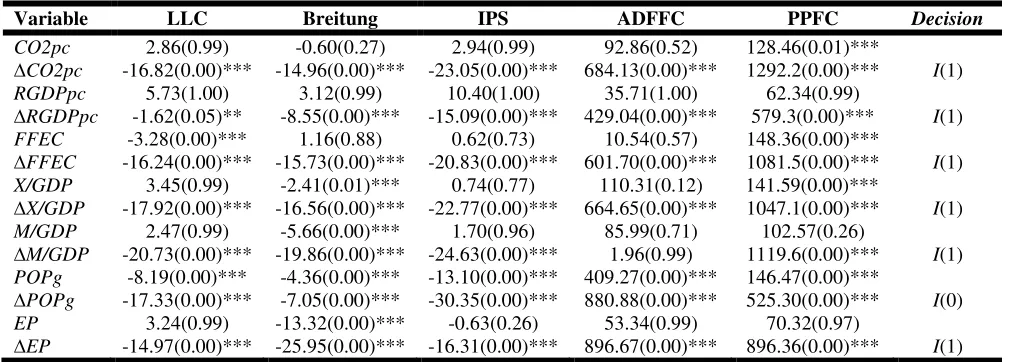
Table 1 presents the unit root test results for each of the variables. Since more than one

panel unit root tests were conducted on the series, a simple majority criterion was employed to

draw conclusion on the order of integration. Overall, as shown in Table 1, apart from population

growth, which was found to be stationary at levels, the result shows that all other variables are

stationary only at their first difference. The I(0) status of population growth is not surprising, since the variable is already measured in growth form.

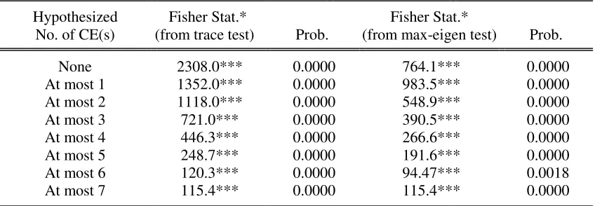
The Johansen Fisher panel cointegration test results are also reported in Table 2. The tests

are performed with one lag. The results show clearly that there is strong evidence of

integration relationship between the variables included in the panel. The presence of

co-integration vectors indicate that the EKC model can be safely estimated with variables in levels

in our sample.

Table 1: Panel Unit Root Test Results

Variable LLC Breitung IPS ADFFC PPFC Decision

CO2pc 2.86(0.99) -0.60(0.27) 2.94(0.99) 92.86(0.52) 128.46(0.01)***

∆CO2pc -16.82(0.00)*** -14.96(0.00)*** -23.05(0.00)*** 684.13(0.00)*** 1292.2(0.00)*** I(1)

RGDPpc 5.73(1.00) 3.12(0.99) 10.40(1.00) 35.71(1.00) 62.34(0.99)

∆RGDPpc -1.62(0.05)** -8.55(0.00)*** -15.09(0.00)*** 429.04(0.00)*** 579.3(0.00)*** I(1)

FFEC -3.28(0.00)*** 1.16(0.88) 0.62(0.73) 10.54(0.57) 148.36(0.00)***

∆FFEC -16.24(0.00)*** -15.73(0.00)*** -20.83(0.00)*** 601.70(0.00)*** 1081.5(0.00)*** I(1)

X/GDP 3.45(0.99) -2.41(0.01)*** 0.74(0.77) 110.31(0.12) 141.59(0.00)***

∆X/GDP -17.92(0.00)*** -16.56(0.00)*** -22.77(0.00)*** 664.65(0.00)*** 1047.1(0.00)*** I(1)

M/GDP 2.47(0.99) -5.66(0.00)*** 1.70(0.96) 85.99(0.71) 102.57(0.26)

∆M/GDP -20.73(0.00)*** -19.86(0.00)*** -24.63(0.00)*** 1.96(0.99) 1119.6(0.00)*** I(1) POPg -8.19(0.00)*** -4.36(0.00)*** -13.10(0.00)*** 409.27(0.00)*** 146.47(0.00)***

∆POPg -17.33(0.00)*** -7.05(0.00)*** -30.35(0.00)*** 880.88(0.00)*** 525.30(0.00)*** I(0) EP 3.24(0.99) -13.32(0.00)*** -0.63(0.26) 53.34(0.99) 70.32(0.97)

∆EP -14.97(0.00)*** -25.95(0.00)*** -16.31(0.00)*** 896.67(0.00)*** 896.36(0.00)*** I(1)

11

Table 2: Johansen Fisher Panel Cointegration Test Trend assumption: Linear deterministic trend

Hypothesized Fisher Stat.* Fisher Stat.*

No. of CE(s) (from trace test) Prob. (from max-eigen test) Prob.

None 2308.0*** 0.0000 764.1*** 0.0000 At most 1 1352.0*** 0.0000 983.5*** 0.0000 At most 2 1118.0*** 0.0000 548.9*** 0.0000 At most 3 721.0*** 0.0000 390.5*** 0.0000 At most 4 446.3*** 0.0000 266.6*** 0.0000 At most 5 248.7*** 0.0000 191.6*** 0.0000 At most 6 120.3*** 0.0000 94.47*** 0.0018 At most 7 115.4*** 0.0000 115.4*** 0.0000

Note: * Probabilities are computed using asymptotic Chi-square distribution, *** denotes significance at 1% level.

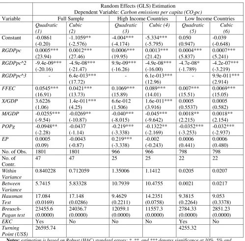
Table 3 shows the estimated results of the relationship between environmental quality

and economic growth. The optimal model selection was guided by the Hausman’s test statistic.

The null hypothesis underlying the Hausman Test is that the random effect model is consistent,

in favour of the fixed effects model. Usually, a low P-values count against the null, while a

higher one counts in support of the null. As can be gleaned from the bottom of Table 3,

especially from columns (3) – (6), we cannot reject the null at the conventional 5% level. Thus,

the random effect model was selected as the optimal model estimation.

Overall, a variety of interesting results emerged from Table 3. When the full sample is

considered, our results in column (1) show that the relationship between environment and growth

follows an inverted U-shape and therefore tends to confirm the EKC-hypothesis with a turning

point at US$ 226596. However, when the cubic term of income per capita is added to the model,

the EKC-hypothesis fails to hold (see column 2). Rather, the evidence shows that the relationship

is described by an N-shaped curve, which exhibits the same pattern as the inverted U-curve initially, but become positive again after a certain income level. This indicates that de-linking

environmental damage from income per capita is only a temporal phenomenon. Similar evidence

have been confirmed in other studies (e.g. Galeotti and Lanza, 1999; Sengupta, 1996;

12

exhausted, or have become too expensive, further income growth will result in net environmental

damage.

Table 3: Environmental Quality and Economic Growth: Random Effects (GLS) Estimation

Random Effects (GLS) Estimation

Dependent Variable: Carbon emissions per capita (CO2pc)

Variable Full Sample High Income Countries Low Income Countries

Quadratic (1) Cubic (2) Quadratic (3)

Cubic (4) Quadratic (5)

Cubic (6)

Constant -0.0861 (-0.20) -1.1059** (-2.576) -4.004*** (-4.174) -5.334*** (-5.795) 0.050 (0.947) -0.039 (-0.648)

RGDPpc 0.0005*** (23.94) 0.0012*** (27.46) 0.0006*** (19.95) 0.0013*** (21.42) 0.0004*** (5.837) 0.0007*** (5.241)

RGDPpc^2 -9.4e-09*** (-20.16) -4.9e-08*** (-21.47) 9.9e-09*** (-16.26) -4.9e-08*** (-16.00) -4.7e-08* (-1.789) -4.2e-07*** (-3.219)

RGDPpc^3 - 6.4e-013*** (17.72)

- 6.1e-013*** (12.96)

- 9.9e-011*** (2.914)

FFEC 0.0545*** (16.91) 0.0421*** (13.73) 0.1069*** (15.89) 0.089*** (14.01) 0.007*** (15.51) 0.0069*** (15.05)

X/GDP 3.6226 (1.06) 1.4e-011*** (4.25) 6.6e-012 (1.506) 1.6e-011*** (3.916) 0.0005 (0.5537) 0.0005 (0.582)

M/GDP -0.0255*** (-9.54) -0.0269** (-10.87) -0.040*** (-8.015) -0.045*** (-9.642) 0.0018** (2.215) 0.0018** (2.154)

POPg -0.0948** (-2.28) -0.0437 (-1.14) -0.219*** (-3.338) -0.1322** (-2.169) -0.0352*** (-3.253) -0.032*** (-2.937)

EP 0.0005

(0.09) -0.0043 (-0.87) 0.219*** (-3.338) -0.002 (-0.243) 0.0006 (0.441) 0.0006 (0.480)

No. of Obs. 1801 1801 966 966 798 798

No. of Contr.

47 47 25 25 22 22

Within Variance

0.840228 0.712059 1.35006 1.1412 0.0205 0.0207

Between Variance

5.7415 5.83328 10.7939 10.4755 0.0021 0.0217

Hausman Test 17.084 (0.0169) 17.148 (0.0286) 9.4629 (0.2211) 14.2351 (0.0758) 9.3815 (0.2264) 9.053 (0.3378) Breusch-Pagan test 23455.6 (0.0000) 24036.7 (0.0000) 12059.1 (0.0000) 11557.3 (0.0000) 2784.33 (0.0000) 2851.23 (0.0000)

EKC Yes No No No Yes No

Turning Point (US$)

26595.74 4255.32

Notes: estimation is based on Robust (HAC) standard errors; *, **, and *** denotes significance at 10%, 5% and 1% respectively. Values in bracket for the estimated coefficient are the t-statistics while those for the F-stats, Hausman and Breusch-Pagan tests are the P-values

When we divide the samples into low and high income countries, an inverted U-shaped

13

from the model (see column 5). With similar restriction, high income countries exhibit an

increasing linear trend. These results conflict sharply with theoretical prescriptions and called for

a re-thinking of the EKC hypothesis. More so, the inclusion of the cubed-income term shows

clearly that EKC is invalid for both high and low income countries. In both cases, the results

returned an N-shaped curve rather than an inverted U-shape.

Going further, the results indicate that fossil fuel consumption is a major culprit in

environmental damage. Expectedly, the impact is significant and much higher in high income

countries than in low income countries. Surprisingly, population growth (though significant)

does not conform to the priori expectations. In the same vain, energy price appears to have no

significant impact on pollution which is inconsistent with theoretical expectations. Perhaps the

unexpected result is because of the distortions in energy prices caused by widespread subsidies

across countries. Given the wide variation in domestic energy prices, the use of one single

measure for the variable may not have been appropriate.

The impact of the trade variables reveals that for the full sample, export is positively

related with environmental damage while import is having the opposite effect. This result is

similar in the case of high income countries. However, for low income countries, the result

shows that both variables are positively related with environmental damage. Clearly, the results

demonstrate that while high income countries are able to curtail environmental damage through

imports, the opposite is the case in low income countries. By extension, it tends to confirm the

pollution haven hypothesis. All else equal, by importing goods to substitute some manufactured

goods that were earlier produced domestically by displaced pollution intensive industries, high

income countries have not only reduce their energy requirements but environmental damage. A

further explanation could be that high income countries are able to introduce new production

process that replaces domestically produced inputs with imported ones.

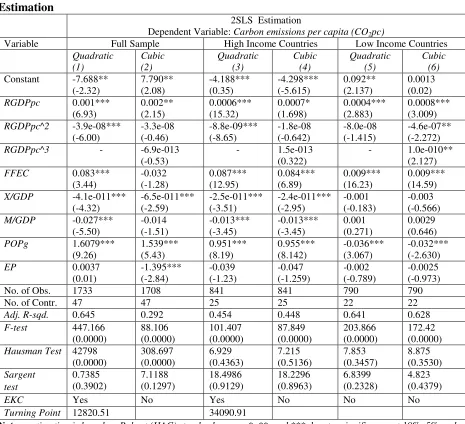
Table 4 contains the results based on two-stage least square estimation that controls for

the feedback effect between income and environmental damage. It was difficult to find

instruments that are both good at predicting the variable of interest and yet are not determinants

of the dependent variable. However, to proceed, we used lagged values of the explanatory

variables as instruments and test their validity using Sargan over-identification test. The null

hypothesis here is that all the instruments are valid. A very low P-value counts against the null in favour of the alternative that they are invalid. Also, we used the Hausman’s test to judge if the

14

IV-method is not necessarily required. Again, a low P-value would counts against the null that OLS estimates are consistent while a high value will support the alternative hypothesis that they

are not. Overall, the results of these diagnostic tests, as shown at the bottom of Table 4, indicate

that the instruments used were valid and that the OLS estimates were inconsistent, except when

the full sample was considered. Because of this, we choose to discuss only the results based on

the sub-samples.

Table 4: Environmental Quality and Economic Growth: Two-Stage Least Square (2SLS) Estimation

2SLS Estimation

Dependent Variable: Carbon emissions per capita (CO2pc)

Variable Full Sample High Income Countries Low Income Countries Quadratic (1) Cubic (2) Quadratic (3) Cubic (4) Quadratic (5) Cubic (6) Constant -7.688**

(-2.32) 7.790** (2.08) -4.188*** (0.35) -4.298*** (-5.615) 0.092** (2.137) 0.0013 (0.02)

RGDPpc 0.001***

(6.93) 0.002** (2.15) 0.0006*** (15.32) 0.0007* (1.698) 0.0004*** (2.883) 0.0008*** (3.009)

RGDPpc^2 -3.9e-08***

(-6.00) -3.3e-08 (-0.46) -8.8e-09*** (-8.65) -1.8e-08 (-0.642) -8.0e-08 (-1.415) -4.6e-07** (-2.272)

RGDPpc^3 - -6.9e-013

(-0.53)

- 1.5e-013 (0.322)

- 1.0e-010** (2.127)

FFEC 0.083***

(3.44) -0.032 (-1.28) 0.087*** (12.95) 0.084*** (6.89) 0.009*** (16.23) 0.009*** (14.59)

X/GDP -4.1e-011***

(-4.32) -6.5e-011*** (-2.59) -2.5e-011*** (-3.51) -2.4e-011*** (-2.95) -0.001 (-0.183) -0.003 (-0.566)

M/GDP -0.027***

(-5.50) -0.014 (-1.51) -0.013*** (-3.45) -0.013*** (-3.45) 0.001 (0.271) 0.0029 (0.646)

POPg 1.6079***

(9.26) 1.539*** (5.43) 0.951*** (8.19) 0.955*** (8.142) -0.036*** (3.067) -0.032*** (-2.630)

EP 0.0037

(0.01) -1.395*** (-2.84) -0.039 (-1.23) -0.047 (-1.259) -0.002 (-0.789) -0.0025 (-0.973)

No. of Obs. 1733 1708 841 841 790 790

No. of Contr. 47 47 25 25 22 22

Adj. R-sqd. 0.645 0.292 0.454 0.448 0.641 0.628

F-test 447.166

(0.0000) 88.106 (0.0000) 101.407 (0.0000) 87.849 (0.0000) 203.866 (0.0000) 172.42 (0.0000) Hausman Test 42798

(0.0000) 308.697 (0.0000) 6.929 (0.4363) 7.215 (0.5136) 7.853 (0.3457) 8.875 (0.3530) Sargent test 0.7385 (0.3902) 7.1188 (0.1297) 18.4986 (0.9129) 18.2296 (0.8963) 6.8399 (0.2328) 4.823 (0.4379)

EKC Yes No Yes No No No

Turning Point 12820.51 34090.91

Notes: estimation is based on Robust (HAC) standard errors; *, **, and *** denotes significance at 10%, 5% and 1% respectively. Values in bracket for the estimated coefficient are the t-statistics while those for the F-stats, Hausman and Sargent tests are the P-values

Generally, in all the estimations, the results show that the presumed EKC ceased to hold

15

cubic term, EKC can be confirmed for high income countries with a turning point at about

US$34091. This closely mirrors what has been found by Cole (2004) who reports a turning point

of US$34880 after controlling for other variables. However, looking at the R-squared, the

relatively low fit of the model (45.4%) portrays that the evidence is (at best) weak. In the case of

the cubic estimation, the EKC typed relationship tends to fade away. These results demonstrate

that relying on a cubic model to validate EKC can generates misleading results and conclusion.

Moving to the low income sample, we found that the entire evidence does not lend strong

supports to the EKC typed relationship. The squared income term in the quadratic model was

insignificant (even though it is negative). The inclusion of the cubic income term confirms the

existence of an N-shaped curve which agrees with the Random effect results in Table 3. In effect, these results tend to demonstrate that decoupling economic growth from environmental damage

is only temporal. It appears that unless cogent measures are taken to protect the environment,

unfettered growth objective would not automatically resolve environmental damage.

Interestingly, most of the control variables conform to their theoretical expectations. For

instance, in almost all the estimations, the impact of fossil fuel consumption on environmental

damage remains positive and significant. As expected, the impact is relatively higher in the high

income sample than in the low income sample. Also, energy prices bear a negative relationship

with environmental damage (though by our results, such impacts are largely insignificant). This

result supports the fact that reforming harmful energy subsidies can contribute (to some extent)

in solving environmental damage. The impact of trade (especially imports) and population

growth shows mixed evidence for high and low income countries. Specifically, for the high

income sample, higher population growth leads significantly to higher CO2 emissions (and

therefore environmental damage) while the reverse is the case in low income countries. For one,

the result could be attributed to energy poverty problem that characterized low income countries.

Energy poverty is a lack of access to modern energy services. Globally over 1.3 billion people

are without access to electricity (IAE, 2013). More than 95% of these people are either in

sub-Saharan African or developing Asia and 84% are in rural areas. Low access translates to low

16

4. Conclusion and Policy Options

The primary motivation behind empirical studies on EKC hypothesis is to search for evidence of

the link between environmental degradation and economic growth so as to answer the relevant

question of whether economic growth alone could serve as a long-run solution to environmental

damage. Similar motivation drives the present study. Here we analyze the relationship using a

panel of 47 countries over the period 1970 -2008. For comparative purpose, apart from pooled

results where all the countries are lumped together, we further divide the sample into high and

low income countries. To resolve the likely simultaneity problem between growth and

environment, we used the two-staged least square (2SLS) estimation technique to correct for the

feedback effect. We tested for the validity and consistency of EKC hypothesis using two

functional forms (quadratic and cubic) and controlled for other key variables that could impact

on environmental quality.

Overall, our findings do not lend strong support to the presumed EKC-typed relationship.

Generally, our result shows clearly that relying on a quadratic model is capable of misleading

researchers to readily ratify the existence of EKC. Further, findings show that EKC hypothesis

ceased to hold whenever an alternative functional form (cubic) is employed. At best the

relationship between economic growth and environmental quality is shown to be typified by an

N-shaped curve - indicating that any delinking of economic growth from environmental quality is temporal. An important policy issue arising from here is that as nations (especially developing

countries) continue to demand more energy to drive their growth process, adequate concern

should be giving to environmental impacts of such process. The evidence in this paper suggests

that it would be misleading to follow the policy of polluting first and cleaning later as espoused

by proponents of EKC. It does not make much sense to “do nothing” and wait for the

magic-wand of economic growth to cure environmental problems. Proactive policies and measures are

required to mitigate the problem.

There are a number of policy instruments for controlling environmental quality. Some of

these include fiscal instruments (e.g. taxes), charge systems (fees), financial instruments (e.g.

subsidies), etc. Alternatively, the state can also use its coercive power to regulate polluter

behavior and limits emissions below a prescribed policy target. A good example here is setting

17

minimum quality of fuels that could be used in production or energy generation purposes may

be specified. In addition, demand-side management options to reduce excessive energy demand

may also be considered (e.g. reforming harmful energy subsidies especially on fossil fuel)

However, the choice of appropriate policy instrument should be considered with respect

to the specific characteristics and conditions of the country as well as the type of environmental

pollutant. In dealing with these issues, policy makers may be guided by the following set of

questions (as in Panayotou, 1994; Bhattacharyya, 2011):

• Environmental effectiveness: Will the chosen instrument achieve the environmental

objective within specified time span and what degree of certainty can be expected?

• Cost effectiveness: Will the instrument achieve the environmental objective at the

minimum possible cost3 to the society?

• Flexibility: Is the instrument flexible enough to changes in technology, the resource

scarcity and market conditions?

• Dynamic efficiency: Does the instrument provide incentive to technological innovation?

Does it promote environmentally sound infrastructure?

• Equity: Will the costs and benefits of the instruments be equitably distributed?4

• Ease of introduction: Is the instrument consistent with the country’s legal framework?

Does it require new legislation? If so, is it feasible? Does the regulatory body have the

requisite administrative capacity to administer the new instrument?

• Ease of monitoring and enforcement: How difficult or costly will monitoring and

enforcement of the instrument be?

• Predictability: The relevant question here is does the instrument combine predictability

and flexibility? Effectiveness of a given policy instrument can be assessed if it remains

in force in the long-run and thus imposes predictable costs on polluters.

• Acceptability: This issue is very important in opting for a particular policy instrument.

The question that needs to be asked here is whether the selected instrument is

understandable by the public, acceptable to the industry and politically saleable.

3

In considering costs to the society, a much wider view should be taken to incorporate those related to compliance, monitoring and enforcement (i.e. administrative cost), as well as any other costs induced by distortions.

4

18

Summing up, evolving a practical solution to the problem of environmental quality requires

a critical assessment of certain issues that relates, amongst others, to its practicability and

effectiveness. While no single instrument may satisfy all the conditions stated above, a

combination of different approaches, specific to the type of pollutant and the circumstances

of the country can be used to ensure that the overall objective of improved environmental

quality is obtained, irrespective of the level of economic growth.

References

Agras, J. and Chapman, D., 1999. A Dynamic Approach to the Environmental Kuznets Curve Hypothesis. Ecological Economics, 28:267-277.

Akpan, G. E. and Akpan, U. F., 2012. Electricity Consumption, Carbon Emissions and Economic Growth in Nigeria. International Journal of Energy Economics and Policy, 2(4): 292-306

Akpan, U. F. and Ekong, C. N., 2013. What are the Growth Effect of Foreign Direct Investment and Trade in WAMZ? European Journal of Business and Management, 5(17): 134-145

Akpan, U.F. and Chuku, C.A., 2011. Economic Growth and Environmental Degradation in Nigeria: Beyond the Environmental Kuznets Curve. In: A. Adinikinju, A. Iwayemiand W. Iledare (Eds),

Green Energy and Energy Security: Options for Africa, 2011 NAEE Proceedings, Pp. 212-234.

Beckerman, W., 1992. Economic Growth and the Environment: Whose Growth? Whose Environment?

World Development. 20(4): 481-496

Bhattacharyya, S. C., 2011. Energy Economics: Concepts, Issues, Markets and Governance.

New York: Springer-Verlag London Limited

Breitung, J., 2002. Nonparametric tests for Unit Roots and Cointegration. Journal of Econometrics, 108(2), 343–363.

Caviglia-Harris, J. L., Chambers, D. and Kahn, J. R., 2009. Taking the “U” out of Kuznets: a Comprehensive Analysis of the EKC and Environmental Degradation. Ecological Economics,

1149-1159.

Choi, I. , 2001. “Unit Root Tests for Panel Data,” Journal of International Money and Finance,

20: 249–272.

Cole, M.A., 2004. US Environmental Load Displacement: Examining Consumption, Regulations and the Role of NAFTA. Ecological Economics, 48(4): 439-450.

De Bruyn, S. M., van den Bergh, J. C., and Opschoor, J. B., 1998. Economic Growth and Emissions: Reconsidering the Empirical Basis of Environmental Kuznets Curves.

19

Friedl, B. and Getzner, M., 2003. Determinants of CO2 Emissions in a Small Open Economy. Ecological

Economics, 45:133-148

Galeotti, M. and Lanza, A., 1999. Desperately Seeking (Environmental) Kuznets. 1998 World Congress of Environmental and Resource Economics, P.46, Venice, 25-27 June

Grossman, G. and Krueger, A., 1991. Environmental Impacts of the North American Free Trade Agreement. Cambridge, MA: NBER.

Grossman, G. and Krueger, A., 1995. Economic Growth and the Environment. Quarterly Journal of Economics, 110 (2), 352–377.

Gujarati, D. and Porter, 2009. Basic Econometrics . McGraw Hill Publishers, New York

He, L. and Richard, P., 2010. Environmental Kuznets Curve for CO2 in Canada. Ecological Economics,

69: 1083-1093

Heil, M. T. and Selden, T. M., 2001. Carbon Emissions and Economic Development: Future Trajectories based on Historical Experience. Environment and Development Economics,

6(1): 63-83

Holtz-Eakin, D. and Selden, T.M., 1995. Stoking the Fires? CO2 Emissions and Economic

Growth. Journal of Public Economics, 57: 85-101

IAE, 2013. World Energy Outlook 2013, available at

http://www.worldenergyoutlook.org/resources/energydevelopment/energyaccessprojectionsto2 030/

Im, K., Pesaran, M., and Shin, Y., 2003. Testing for Unit Roots in Heterogeneous Panels.

Journal of Econometrics, 115(1), 53–74.

Levin, A., Lin, C.F. and Chu, C. S. J., 2002. Unit Root Tests in Panel Data: Asymptotic and Finite-Sample Properties, Journal of Econometrics, 108(1): 1 – 24

Maddala, G. S. and S. Wu, 1999. A Comparative Study of Unit Root Tests with Panel Data and a New Simple Test. Oxford Bulletin of Economics and Statistics, 61: 631–52.

Matinez-Zerzoso, I. and Bengochea-Morancho, A., 2004. Pooled Mean Group Estimation for an Environmental Kuznets Curve for CO2. Economic Letters, 82: 121-126

Munasinghe, M., 1999. Is Environmental Degradation an Inevitable Consequence of Economic Growth: Turning Through the Environmental Kuznets Curve. Ecological Economics, 29: 89-109

Panayotou, T., 1993. Empirical tests and Policy Analysis of Environmental Degradation at different stages of Economic Development. Geneva: International Labor Office, Technology and Employment Programme

Panayotou, T., 1994. Economic Instruments for Environmental Management and Sustainable Development. UNEP Paper 16, UNEP, Nairobi

20

Phillips, P. and Perron, P., 1988. Testing for a Unit Root in Time Series Regression, Biometrica, 75 (2): 335-346.

Sengupta, E., 1996. CO2 Emission-Income Relationship: Policy Approach for Climate Control. Pacific

and Asian Journal of Energy, 7: 207-229.

Shafik, N. and Bandyopadhyay, S., 1992. Economic Growth and Environmental Quality: Time Series and Cross-Country Evidence. Background Paper for the World Development Report 1992, the World Bank, Washington DC

Stern, D. I., 2004. The Rise and fall of the Environmental Kuznets Curve. World Development, 32: 1419-1439

Stern, D.I., Common, M.S., Barbier, E.B., 1996. Economic growth and environmental degradation: a critique of the environmental Kuznets curve. World Development, 24: 1151–1160.

World Bank, 2012. World Development Indicators/Global Development Finance, the World Bank, Washington DC

Appendix

Table A1: Data Construction and Sources

Variable Definition/Measurement Source

CO2pc

Carbon-dioxide emissions (measured in metric tons per capita) are those stemming from the burning of fossil fuels and the manufacture of cement. They include carbon dioxide produced during consumption of solid, liquid, and gas fuels and gas flaring.

WDI/GDI database, 2012

RGDPpc Real GDP per capita (measured in constant 2000 US$)

WDI/GDI database, 2012

FFEC

Fossil fuel consumption (measured as a % of total fuel consumption)comprises consumption of coal, oil, petroleum, and natural gas products.

WDI/GDI database, 2012

EP

Real World Oil Price based on OPEC Reference Basket (i.e. Nominal Oil Price Adjusted for Exchange Rates and Inflation), using 1973 as the base year. The variable is measured in US dollars per barrel (US$/b)

OPEC database, 2012

POPg

Annual population growth rate

WDI/GDI database, 2012

X/GDP

Exports of goods and services represent the value of all goods and other market services provided to the rest of the world. The variable is expressed in percentage of GDP

WDI/GDI database, 2012

M/GDP

Imports of goods and services represent the value of all goods and other market services received from the rest of the world. The variable is measured as a percentage of GDP

WDI/GDI database, 2012

21

Table A2: Summary Statistics of the Variables

CO2pc RGDPpc FFEC X/GDP M/GDP POPg EP Mean 4.9339 8418.4 60.248 1.2e+009 33.759 1.7075 7.9088 Median 2.5969 2498.7 63.072 27.352 29.640 1.7471 6.6430 Minimum 0.0294 82.672 2.7067 2.6097 2.7045 -1.6096 2.3960 Maximum 22.511 41904 100.25 1.7e+011 219.07 6.3610 16.125 Std. Dev. 5.2314 10108 30.403 1.1e+010 24.193 1.1754 4.1214 Skewness 1.0027 1.1336 -0.24919 10.793 3.9305 0.2987 0.6856 Kurtosis 3.24830 3.28039 1.6000 133.59 23.656 2.9128 2.2707 C.V. 1.0603 1.2007 0.50463 8.5398 0.7167 0.6884 0.5211

Obs. 1831 1828 1806 1828 1828 1833 1833

Table A3: Correlation Matrix of the Variables

CO2pc RGDPpc FFEC EP POPg X/GDP M/GDP

CO2pc 1.0000

RGDPpc 0.7616 1.0000

FFEC 0.6704 0.4405 1.0000

EP -0.0173 0.0069 -0.0070 1.0000

POPg -0.4239 -0.5206 -0.4479 0.0217 1.0000

X/GDP 0.0674 0.1593 0.0683 0.0151 -0.1320 1.0000

M/GDP 0.0941 0.0551 0.1498 0.0834 0.0414 0.0420 1.0000

Table A4: Countries included in the sample

High Income Countries Low Income Countries

Norway, Korea Republic, Japan, Australia,

Portuguese Republic, Italy, Austria, Saudi

Arabia,

Canada,

Hungary,

Iceland,

Portuguese

Republic,

Chile,

China,

Cyprus,

Denmark,

Finland,

French

Republic,

Hellenic

Republic,

Israel,

Singapore, South Africa, Sweden, United

Kingdom and United States

Philippians,

Nigeria,

Bangladesh,

Benin, Bolivia, Cameroon, Democratic

Republic of the Congo, Republic of

Congo, Côte d'Ivoire, El Salvador,

Ghana, Honduras, India, Indonesia,

Kenya, Morocco, Pakistan, Paraguay,

Senegal, Sri Lanka, Sudan and Togo

22

0 5 10 15 20 25

0 5000 10000 15000 20000 25000 30000 35000 40000

C

O

2

e

m

is

s

io

n

s

p

e

r

c

a

p

it

a

(

C

O

2

p

c

)

Real GDP per capita (RGDPpc)

Fig. AI: CO2 emissions per capita (CO2pc) versus Real GDP per capita (RGDPpc) (with quadratic fit)