Applications of microcomputers in interactive image processing

IN INTERACTIVE I~lliGE PROCESSING

A thesis

presented for the Degree of

Doctor of Philosophy in Electrical Engineering

in the

University of Canterbury Christchurch, New Zealand

by

ABSTRACT

Interactive image processing systems are reviewed and a system incorporating a charge coupled device imaging array, a microprocessor computing element, and a real time image display is described. Applications are given,

including the description of a system capable of collecting multispectral images for satellite imagery calibration.

A new technique, called shift and add, which allows nearly diffraction limited images to be formed of objects viewed through a randomly distorted, turbulent media is formulated. The successful simulation of the method in an optical laboratory is reported. Results are given which show that if the method is applied in large telescope, optical astr.onomidal imaging, nearly di ffraction limited

I am deeply grateful to Professor R.H.T. Bates, my colleague and supervisor, for his help, encouragement and guidance during the course of the project. Professor Bates negotiated the initial contract for research into solid state sensors which led to the development of the University of Canterbury Image Processing System. The development of the image processing hardware has been a joint effort with Dr R.M. Hodgson. To him goes my

gratitude for taking care of research contract reports and for helping make the decisions which led .to our useful image processing system. Mr W.K. Kennedy, also, was

especially active in this area during the early design phases. I acknowledge the immense contribution to the hardware and software design and construction made by post-graduate students A.J. Ireland, G.A. Duncan,

J.K.N. Murphy, D. Pairman, M.A. Rodgers and C.B. Lake. Without their enthusiastic help the system would still be very primitive. I extend many thanks to the rest of my colleagues in the Electrical Engineering Department, especially to Mr W.K. Kennedy, for putting up with my recent dedication to this task to the detriment of some of my other duties.

This thesis is much better for the proof-reading and English corrections made by my wife Katie.

CONTENTS Page Abstract Acknowledgements Glossary i ii xi

Preface xx

CHAPTER 1 : INTERACTIVE IMAGE PROCESSING SYSTEMS 1.0 Introduction

1 1 4 5 6 9 1.1 Interactive Digital Image Processing

1.1.1 Imaging Systems Analysis 1.2 Image Conversion System

1.2.1 Image Formation

1.2.2 Image Characterization

(a) Spectral characteristics (b) Intensity

(c) Contrast

(d) Dynamic range

(e) Spatial frequency content 1.2.3 Image Detectors

(a) Quantum efficiency (b) Sensitivity

(c) Spectral response (d) Noise

11 12 12 12 13 13 16 17 18 18 19

(e) Dark signal 19

(f) Fixed pattern noise 19

(g) Readout noise 19

(h) Dynamic range 20

(i) Signal-to-noise ratio 20

(j) Detective quantum efficiency 20

(k) Gamma 22

(1) Linearity 23

(m) Geometrical effects 23

(n) Modulation transfer function 24 1.2.4 Analog-to-digital Conversion 27

1.3

(b) Aperture time (c) Conversion time (d) Resolution

(e) Sample-and-hold Digital Processing System

1.3.1 Image Processing Characterization (a) Algorithm

(b) Accuracy

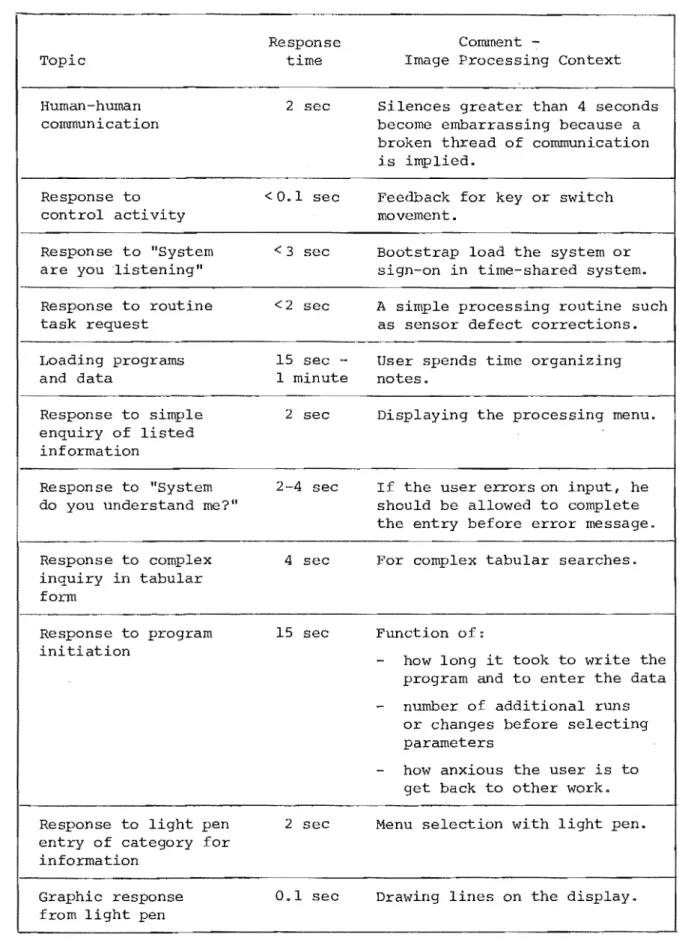
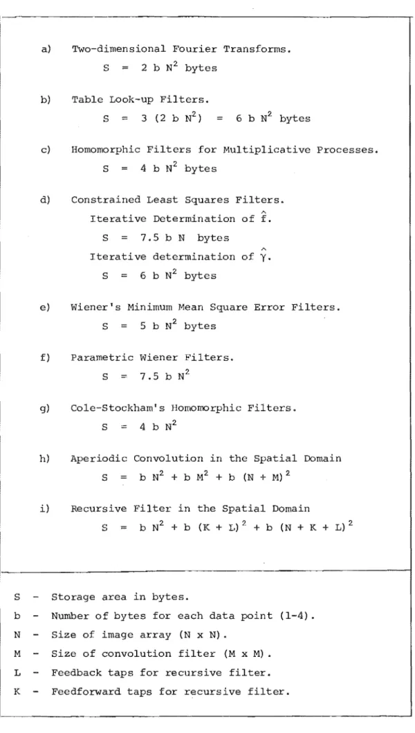
1.3.2 What is the Processing Time Limit

Page 28 29 29 29 30 31 31 32

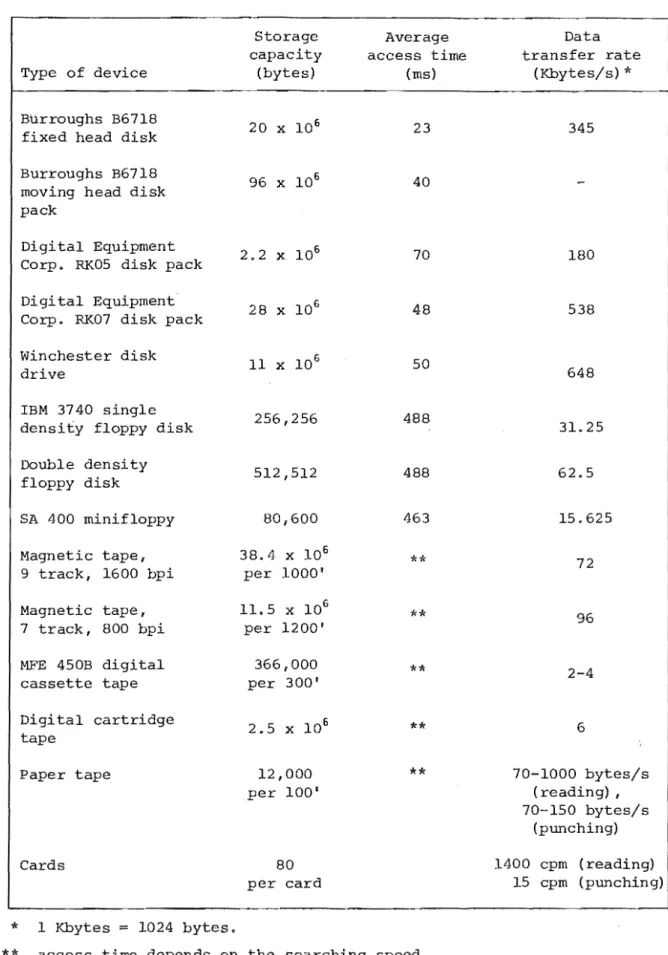
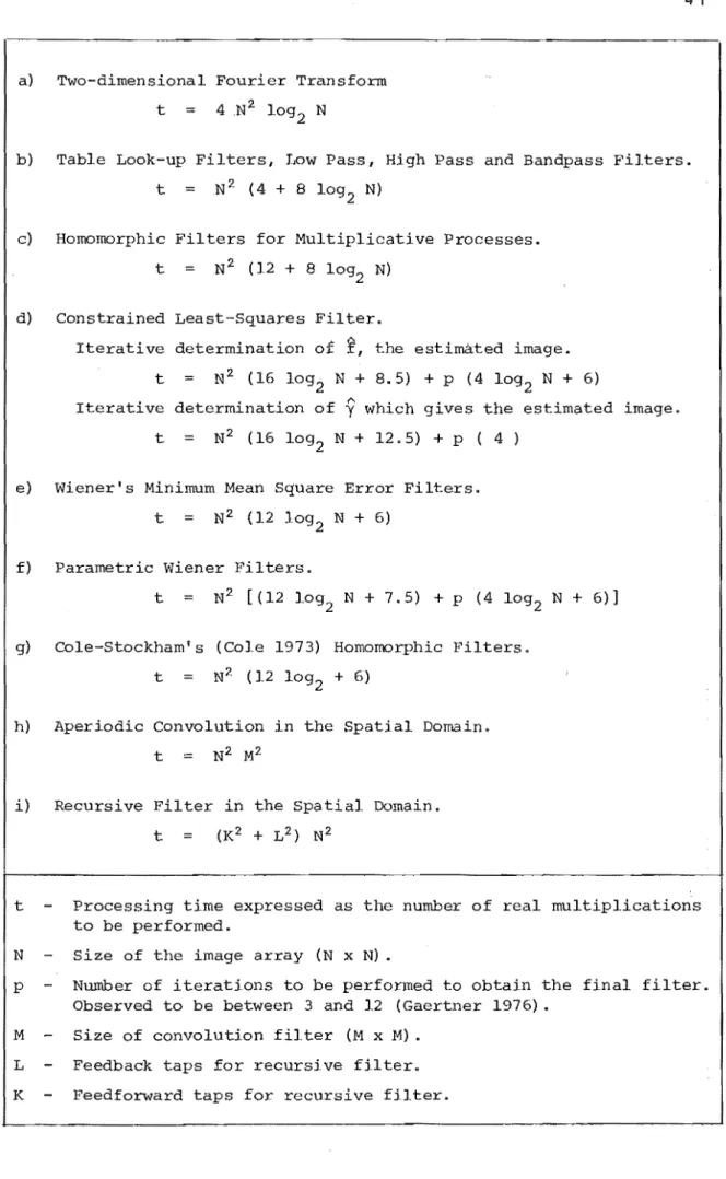
for Interactive Image Processing? 35 1.3.3 Analysis of Image Processing

Time and Storage 37

1.4

(a) Data input

(b) Processing time (c) Processing storage (d) Data output

Image Display

1.4.1 Digital-to-analog Conversion (a) Accuracy

(b) Resolution (c) Settling time (d) Glitches

1.4.2 Display Characteristics (a) Luminance

(b) Contrast ratio (c) Resolution

(d) Geometric fidelity (e) Flicker

(f) Persistence

1.4.3 Image Display Devices 1.4.4 Hard Copy Techniques 1.5 Conclusion

CHAPTER 2: A MICROPROCESSOR BASED INTERACTIVE IMAGE PROCESSING SYSTEM

2.0 Introduction

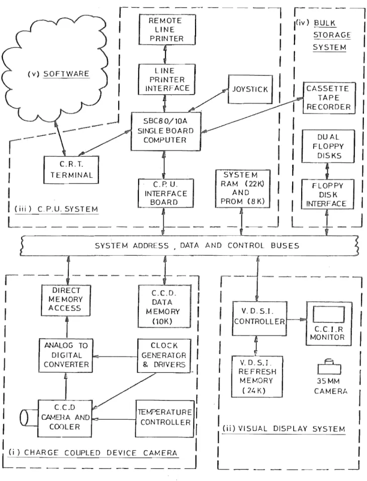
2.1 University of Canterbury Image Processing System (UCIPS) Overview

2.2

2.1.1 Charge Coupled Device Camera and Associated Circuitry

(a) CCD Camera and

temperature controller

Page

54 54 (b) Clock generator and drivers 56 (c) Analog-to-digital converter 56 (d) Direct Memory Access

(DMA) controller 57

(e) CCD Data memory 2.1.2 Visual Display System

(a) Visual display store interrogator (VDSI) (b) VDSI refresh memory (c) Display hard copy 2.1.3 Central Processor unit

System Architecture

(a) Central processor unit (b) Single board

computer interface (c) Cathode ray tube (CRT)

console terminal

(d) Line printer interface (e) Joystick

(f) System RAM and PROM (g) System input/output 2.1.4 Bulk Storage System

(a) Dual floppy disk system (b) Digital cassette

2.1.5 Software

(a) Operating system software (b) User's software

Interactive Image Processing Software 2.2.1 PIKKY - Picture Processing

Operating System

(a) PIKKY command input and decoding

(b) PIKKY floppy disk handling routines

(c) Image processing routines in PIKKY

2.3

2.2.2 External Image Processing Routines 2.2.3 Evaluation of Image

Processing Software

Applications of the University of Canterbury Image Processing System 2.3.1 Flying FADS System

2.3.2 Evaluation of Image Processing Procedures 2.3.3 Astronomical Imaging 2.3.4 Microscope Imaging

2.3.5 General picture Digitization

Page 75 79 81 81 83 88 88 89

2.4 Conclusion 89

CHAPTER 3: THE CHARGE COUPLED DEVICE IMAGING ARRAY 90

3.0 Introduction 90

3.1 Solid State Self Scanned Sensors 90

3.2

3.1.1 Charge Packet Generation 3.1.2 Charge Transfer

CCD202 Characteristics

3.2.1 Physical Architecture

3.2.2 Electrical Characteristics

92 93 96 96 98

(a) Quantum efficiency 98

(b) Sensitivity 99

(c) Spectral response 99

(d) Dynamic range 100

(e) Signa1-to-noise ratio 100

(f) Detective quantum efficiency 101

(g) Dark signal 101

(h) Fixed pattern noise 101

(i) Readout noise 101

(j) Gamma and linearity 102

(k) Modulation transfer function 103

(1) Blooming 104

3.3 Conclusion 105

CHAPTER 4: OPTICAL ASTRONOMICAL IMAGING 4.0 Introduction

4.1 High Resolution in Astronomy

4.2 4.3 4.4 4.5 4.6 4.7 4.8 4.9 4.10

4. 11 4.12

4. 13

Page

4.1.1 Astronomical Imaging 109

(a) The transmission function 109 (b) Quasimonochromatic radiation 109

(c) Exposure time 110

(d) Isoplanacity 111

4.1. 2 4. 1 .3 4.1.4

Diffraction Limited Imaging Angular Resolution

The Effect of the Atmosphere

112 114 116

(a) Exposure time 117

(b) Isoplanacity 117

(c) Transmission function 118

(d) Modulation transfer function 118 Speckle Interferometry (Labeyrie)

Large Field Speckle Interferometry (Liu and Lohmann)

Speckle Holography

(Bates, Gough and Napier) Knox and Thompson Algorithm Lynds, Worden and Harvey Method Speckle Masking (Weigelt)

Autocorrelation, Cross-correlation Subtraction (Worden)

Bates and Milner Speckle Mask and Correlation Processing Fienup Algorithm

CLEAN (Hogbom)

A Stochastic Image Restoration Procedure (Bates)

Other Processing Methods

(a) Michelson Interferometry (b) The Intensity Interferometer (c) Phase Flipping

(d) Stellar Interferometry with a Prominent Variable

120 124 126 129 131 135 139 143 145 149 155 157 157 158 159

4.14 Discussion and Conclusion

160 161

CHAPTER 5: A NEW METHOD TO RECONSTRUCT DIFFRACTION LIMITED IMAGES 5.0 Introduction

5.1 Speckle Shift and Add Processing

163 163

5.2 Experimental Procedures

5.2.1 The Optical Laboratory

Page 169 171

5.2.2 Spatial Incoherency 173

5.2.3 Relative Intensities of the Stars 175 5.2.4 Shift and Add Algorithm

Implementation 178

5.3 Conclusion 180

CHAPTER 6: EXPERIMENTAL RESULTS OF

SHIFT AND ADD PROCESSING 181

6.0 Introduction 181

6.1 Imaging Star Clusters 183

6.2 Point Spread Function for Shift and Add 183 6.3 Calibration of Shift and Add Processing 185

6.3.1 Relative Intensities 185

6.4

6.5

6.6

6.7

6.8

6.3.2 Ghost Stars

The Simulation of Wide Band Speckle Imaging

6.4.1 Wide Band Speckle Results Shift and Add Processing in the Presence of Severe Aberrations 6.5.1 Results of Imaging with a Defocussed Instrument Shift and Add Processing with Wide Band Radiation and Severe Aberrations

Imaging an Extended Object

6.7.1 Imaging an Extended Object with a Defocussed Instrument 6.7.2 An Extended Object with

Wide Band Light Use of the Method CLEAN

6.8.1 CLEAN with Star Clusters

6.8.2 CLEAN with an Extended Object 6.9 Imaging with a Multiple Aperture 6.10 Other Shift and Add Characteristics

and Results

6.10.1 Contrast Improvement by Increasing the Number of Iterations of Shift and Add 6.10.2 Background Noise

Page

6.10.3 Other Extended Objects 6.11 Discussion of Results

CHAPTER 7: CONCLUSIONS AND SUGGESTIONS FOR FURTHER RESEARCH

7.0 Introduction

7.1 Further Shift and Add Processing Experimental Work

7.2

7.3

REFERENCES

7.1.1 Extended Objects 7.1.2 Aberrations

7.1.3 Wide Band Simulations 7.1.4 Ghosts

7.1.5 Inverse Filtering

7.1.6 Solar Speckle Shift and.Add Practical Application of the

Shift and Add Method 7.2.1 Implementation

(a) Choice of sensor

(b) Computational facilities (c) Data storage

7.2.2 Optic Instruments 7.2.3 Shift and Add with

Other Techniques Conclusion

APPENDIX A1: CCD202 100x100 Element Area

210 210 214 214 214 215 215 215 216 217 217 218 219 219 220 221 222 222 224 225

Image Sensor Charge Coupled Device 248

APPENDIX A2: Calculation of CCD202 performance 254

APPENDIX B: University of Canterbury

Monitor Commands 255

APPENDIX C: Interactive Image Processing Software 259

APPENDIX D1: Structure diagram for shift and add 271 D2: Operating Shift and Add software 276 D3: Operating instructions for

CLEAN and ECLEN 278

APPENDIX E: Experimental Conditions for

Results given in Chapter 6 281

APPENDIX F: Experimental Calculations 282

y

b.Q 2

o

b.t b.V £

r;,n

e

pm

v

p

GLOSSARY

Scaling factor in CLEAN.

Transfer characteristic of film. Region of error in Feinup algorithm. Dirac delta function.

Bandwidth.

Range frequencies in a nite bandwidth. Array of delta functions.

Estimate of b. (.)

Array of delta functions at the centres of the bright speckles in a speckle image. Fourier transform of b. (0)

n Change in density of film. Differences in path length.

Mean square fluctuation at the input of a detector.

Mean square fluctuation at the output of a detector.

Coherence time.

uncertainty in input voltage.

One-dimensional spatial frequency phase. Cartesian coordinates in object plane. Angular separation.

Mean wavelength. Microjoules. Micrometres.

T

a ( . ) a

n

A ( • )

A

AID

ASCII

ATR b b ( • )

B ( • )

c

summation.

Short exposure time interval. CCD horizontal clock waveform. CCD photogate clock waveform. CCD vertical clock waveform.

Phase of optical trans function.

Multiplicative constant in Fienup algorithm. One-dimensional spatial frequency.

Point spread function of limited aperture. Location of the brightest point in a

one-dimensional speckle image. Fourier transform of a(·). Area of one pixel in CCD. Analog-to-digital.

American Standard Code for Information Interchange.

Analog transport register.

Number of bytes per data point.

Point spread function due to aberrations in a receptor.

Fourier transform of b(o). Speed of light.

Celsius.

Contrast for dark targets. Contrast for light targets. Contrast as modulation. Valid command in PIKKY. Contrast ratio.

CCD CID cm CP/M CPU CRT CTF D DB DM DMA D.S.I.R. DQE

E 2

F

E 2

o exp f ( • )

FADS FDOS FFT FT

F

g

Charge Coupled Device. Charge Injection Device. Centimetre.

Control Program Monitor floppy disk operating system.

Central processor unit. Cathode ray tube.

Contrast transfer function. Diameter receptor.

Density of film. Digital-to-analog. Dirty beam.

Dirty map.

Direct memory access.

Department of Scientific and Industrial Research. Detective quantum efficiency.

Mean square error criteria in Fourier domain. Mean square error criteria in object domain. Exponential.

True image resolved to the diffraction limit. Maximum frequency.

Total diffraction limited object consisting

of an extended object and an unresolvable object. Fast Area Digitizing Scanner.

Floppy Disk Operating System. Fast Fourier Transform.

Fourier Transform.

g ( • )

h

h ( 0 )

h (.)

n

H H ( • )

H

(Ii)

i ( . )

iL ( .) in ( . ) I (.)

n I/O j J k K

K bytes kg

1 ( . ) L

True diffraction limited image convolved with the average speckle.

Estimate of g(o).

Members of an ensemble of random processes. CCD horizontal clock period.

Point spread function.

Point spread function at the time of the nth speckle image.

Point spread function of shift and add process. CCD vertical clock period.

Fourier transform of h(·). Fourier transform of

h(·).

Intensity distribution in image plane. Long time exposure image.

Nth speckle image.

Fourier transform of i (o).

n

Brightest point in a dirty map. Input/Output.

Autocorrelation of i (o).

n

Joule.

Wave number.

Feedforward tape for recursive filter. 1024 bytes.

Kilogram.

Line spread function.

Feedback tap for recursive filter. Maximum luminance.

Lb Background luminance. L _c Coherence length. L

0 Average luminance.

L_t Target luminance.

LSB Least significant bit.

mV Millivolts.

M.

ln Input modulation. M x M Spatial filter size.

M(w) Modulus of optical transfer function. mHz Megahertz.

MIS Metal insulator-semiconductor.

mm Millimetre.

ms Millisecond.

MTF Modulation transfer function. n Number of bits in a digital word. n

p Number of photons.

N Noise.

'"

N Noise plus the less bright speckles. N x N Size of an image.

nm Nanometres.

ns Nanoseconds.

0(· ) Intensity distribution in object plane.

o ( .)

Fourier transform of 0(0). otf Optical transfer function. Pn Parameter in PIKKY command. p ( • ) Shift and add processed image. p ( .. ) _{Fourier transform of p(o) •}

psf psi q ( • ) Q QE r r o R RMS s -S SI sipsf SNR t T tAP t cy T (w)

" u v U u,v U(x,y)

Point spread function. Point spread invariant. Transmission function. Quanta.

Quantum efficiency.

Number of bits in the exponent. Average size of a seeing cell. Mean output level of a detector. Relative intensity ratio.

Random access memory. Root-mean-square.

Number of bits in the mantissa. storage area in bytes.

Saturation exposure.

Intensity of kth speckle.

Imaginary part of the optical transfer function. Speckle Interferometry.

Spatially invariant point spread function. Ratio of partial scale signal to noise. Processing time.

Redistribution time of the atmosphere. Aperture time.

Memory cycle time.

Optical transfer function.

Spatial frequency where A(u,v) has signi cant value.

Seeing limited frequency.

UCIPS UCSD V V

M

V N

V RMS

V SAT

V T

VDSI W

x,y

z

8

(

.

)

<CR> <ESC> <ETX>

University of Canterbury Image Processing System. University of California at San Diego.

Volts.

Maximum voltage amplitude. Noise voltage.

RMS value of noise voltage. Saturated output voltage. Total noise voltage.

Visual Display Store Interrogator. Watts.

Cartesian coordinates in image or observation plane.

Distance between aperture and observation plane. Correlation operation.

Convolution operation.

One or two dimensional parameters. Ensemble average.

Carriage return keystroke. Escape keystroke.

"When you take stuff from one writer, it's plagiarism;

but when you take it from many writers, it's research."

Preface

APPLICATIONS OF MICROCOMPUTERS IN INTERACTIVE IMAGE PROCESSING

Microprocessors and other large scale integrated circuit devices are having a profound effect on many fields of activity, including digital image processing. The latter is normally performed with expensive, large scale equipment but the recently developed solid state imaging array, combined with the microprocessor as a computing element, can lead to low cost but dramatically effective image processing equipment.

Any digital image processing system can be subdivided into three parts. These are:

(i) the digitization of the image,

(ii) the performance of an image processing calculation or transformation, and (iii) the display of the processed image.

Rapid technological advances are occurring in each of these areas. Input transducers for image processing are now being fabricated as two dimensional arrays of sensors using integrated circuit technology. For example, a 400x400 element charge coupled device imaging array with a

resolution of 20 line pairs per millimetre has been constructed (Smith 1976). Charge coupled devices have dynamic ranges of up to 1000:1, possess quantum

The processing of images can be done with microprocessor computing elements. These large scale integrated circuits will soon have up to 100,000 transistors per chip (Capece

1978) and are rapidly increasing in computer power. Shepard (1977) has predicted that a thirty-two bit

microprocessor will soon be available on a single chip. The processed image is usually displayed with conventional television techniques, often in colour, which is used

either as an alternative method of distinguishing between gray levels (false colour) or as a means of presenting multispectral imagery (e.g. using data gathered by satellites) .

In this thesis digital image processing is approached from the viewpoint of using simple image processing

equipment in an interactive manner. Chapter 1 reviews interactive image processing systems, discussing the image chain from the original object, through the sensor, the digital processing stage, and finally to the display of the processed image. Interactive image processing requirements are considered. Chapter 2 illustrates a stand-alone

microprocessor and charge coupled device (CCD) interactive image processing system that has been developed in our laboratory. Our approach to utilizing real-time image capture and microprocessor-based computing seems to differ significantly from what has been developed elsewhere.

an earth resources sensing satellite (Landsat). The-performance of the charge coupled device sensor used in the image processing system is discussed in detail in Chapter 3.

The image processing system described in Chapter 2 has been used to develop and evaluate image processing techniques which form a diffraction limited image of an object viewed through a randomly turbulent media. This problem is exemplified by the imaging of celestial objects with large earthbound telescopes. The image processing system is used to acquire images in real time from an optical laboratory simulation. A review of techniques which can form diffraction limited images in optical

astronomy is presented in Chapter 4. Chapter 5 describes a method developed jointly with Prof. Bates which extends the processing techniques of Bates and Milner (1979) and allows images to be formed with nearly diffraction limited accuracy. Chapter 6 presents results that have been

achieved when using this new process in astronomical

imaging simulations. Chapter 7 concludes with a discussion of the implementation of the method in actual astronomical imaging. The author's contribution to this new imaging

method has been in generating test simulations and exploring the limitations and characteristics of the methods described.

It is appropriate here to acknowledge the "student powerl1

described in Chapter 2. As a full time member of the academic staff of the Electrical Engineering Department, University of Canterbury, part of my duties included the supervision of final year and postgraduate student projects.

(Note that in American parlance a postgraduate student is a graduate student.) A list of these is given in Appendix G and specific acknowledgement is given in the text where appropriate. Postgraduate students Ireland (1977), Duncan

(1978), Murphy (1979) and Pairman (1980) contributed much to the hardware design and construction of the system. My primary function during this stage of development was to serve as chief engineer and to help overall progress.

A number of papers describing the imaging system, its uses, and the new method developed for processing astronomical image data have been published or are in preparation. These include:

Cady, F.M. and Bates, R.H.T. "Speckle processing gives diffraction limited true images from severely

aberrated instruments," Optics Letters. submitted for publication April 1980.

Bates, R.H.T. and Cady, F.M. "Towards true imaging by wideband speckle interferometry," Opt. Commun. Vol. 32, No.3, 1980, pp. 365-369.

Cady, F.M., Hodgson, R.M., Ireland, A.J. and Duncan, G.A. "A CCD based image processing system," NZIE Proc. Tech. Groups, Vol. 4, No. 2E(ETG), 1979.

Cady, F.M., Pairman, D. and Hodgson, R.M. "PIKKY - A

Hodgson, R.M., Cady, F.M. and Murphy, J.K.N. "The

development of a multispectral scanner to be flown in a ght aircraft," Proc. Landsat 79, 1st.

Australasian Landsat Conference, May 22-25, 1979, Sydney, Australia.

Cady, F.M. and Hodgson, R.M. "A microprocessor based interactive image processing system," lEE Journal of Computers and Digital Techniques. submitted for publication January 1980.

Hodgson, R.M. and Cady, F.M. "Remote sensing from ght aircraft using solid state arrays,1I Photogrammetric Engineering & Remote Sensing. submitted for

publication January 1980.

Cady, F.M., Hodgson, R.M., Pairman, D., Rodgers, M. and Atkinson G.J. "Interactive image processing software

for a microcomputer," in preparation for lEE Journal of Computers and Digital Techniques.

Cady, F.M., Bates, R.H.T. and Berzins, G. through fluctuating distorting media.

"Imaging

I Experimental techniques and image processing applications;

II Theory of speckle interferometry and its extensions; III The shift and add procedure;

CHAPTER 1

INTERACTIVE IMAGE PROCESSING SYSTEMS

1.0 INTRODUCTION

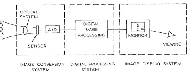
An interactive image processing system, as

illustrated Figure 1.1, consists of three major

sub-systems. These are the image conversion system which

converts the two dimensional image to an array of digital

words, the digital processing section which performs some

transformation of the picture data, and the image display

system which presents the processed image for viewing by

the operator of the image processing system.

1

-I

OPTICAL

I

SYjTEM

- - - I , - - -

- - - I

I

I

I

DIGITAL

I I

r--II

I

IMAGE

~I--'-I

- I

i l i _

~

I

PROCESSING

I

I

MONITOR --~

I

1 SENSOR I I

I

I VIEW!NG

'!

L ____

~

L ____

~

L _ _ _ _ _ _

...J

IMAGE CONVERSION DIGITAL PROCESSING IMAGE DISPLAY SYSTEM

SYSTEM SYSTEM

Image processing terminology tends to be used in slightly different ways by different authors. Green (1977) suggests that there are two broad categories of image

processing. These are the subjective enhancement and the quantitative enhancement of images. Subj ecti ve enhancement is designed to re-display image data for viewing by a human observer. Particular qualities or features of the image

are enhanced to allow optimal interpretation by the observer. These enhancement techniques are usually performed in an

interactive manner to allow the viewer to find an optimum strategy_ Quantitative enhancement, on the other hand, is based on some mathematical model and is not normally an interactive procedure. Quantitative enhancement techniques include geometrical transformations to correct for optical distortion in the picture recording process and the removal of defects caused by the input transducer (Bernstein 1976: Van Wie and Stein 1977). Other authors (Huang 1975;

McDonnell 1975; Andrews and Hunt 1977) distinguish between the terms restoration and enhancement. Restoration refers to processing which is designed to reconstruct an image that has been degraded by some process. Enhancement is an attempt to improve the appearance of the image for human viewing. Restoration techniques include geometrical transformations and defect corrections mentioned above. They also encompass those techniques by which the degrading process, such as blurring, is represented by a mathematical model. An attempt is made to restore the degraded image by applying the inverse of the degrading process. The term

Mersereau 1974; Lewitt and Bates 1978). This term is used to describe the production of an image from data which is generated or gathered in a transform plane, e.g. the Fourier transform plane. Examples of this kind of image

reconstruction are found in computer aided tomography (CAT) scanners (Peters 1973; Bates et aZ. 1975) and synthetic aperture imaging systems (Tomiyasu 1978).

A combination of these similar views and terms seems appropriate. It is convenient to consider techniques

grouped according to their suitability for use in an

interactive image processing situation. Some techniques may be used to restore an image interactively, particularly when the degradation process is not well understood and

parameters must be varied to obtain the 'best' image.

Other techniques may be used in a batch mode of operation. This is often the case when the results of a processing step, e.g. the geometrical rectification of non-linear scanning distortions, are well understood and must be

applied before other processing is undertaken. Batch mode operations are also used when the processing is lengthy or requires considerable computational power as in a Fast Fourier Transform (FFT).

predominately the time spent by the program waiting in the job queue. Elapsed time, along with the amount of storage required, can be used to determine if image processing procedures can be performed interactively, and if the

equipment upon which the processing will be carried out is suitable. These factors are considered in more detail in

§ 1. 3.

Interactive digital image processing is reviewed in this chapter. The concept of an imaging system is discussed and the limits of interactive image processing are defined. The component subsystems, including the image conversion system (§1.2), the digital image processing procedures

(§1.3), and the display and hard copy of the processed image (§1.4) are also discussed.

1.1 INTERACTIVE DIGITAL IMAGE PROCESSING

Interactive digital image processing can be

For the purposes of the following discussion, an interactive digital image processing system is defined to include the following:

(i) A means of digitizing an image in the visible or near-infrared wavelength bands. This restriction is made because the following sections deal with sensors which are active in the visible to near-infrared wavelengths. Other types of sensors, . such as those sensitive to thermal or x-radiation,

are not discussed. The production of images by

synthetic aperture techniques is also not discussed. (ii) A digital processing element. This thesis is

based on the use of microcomputers in image processing and specific examples of their use

are given. A further limitation is imposed to limit the discussion to dedicated systems rather than to include time sharing systems.

(iii) A method of di Various techniques are reviewed and i t is shown that the display of images, and particularly the hard copy of images, is an area in which technological advances need to be made.

1.1.1 Imaging Systems Analysis

(i) the image conversion system which converts the desired input image into a digital representation, (ii) the processing applied to the input image information,

and

(iii) the output or display of the resultant processed image.

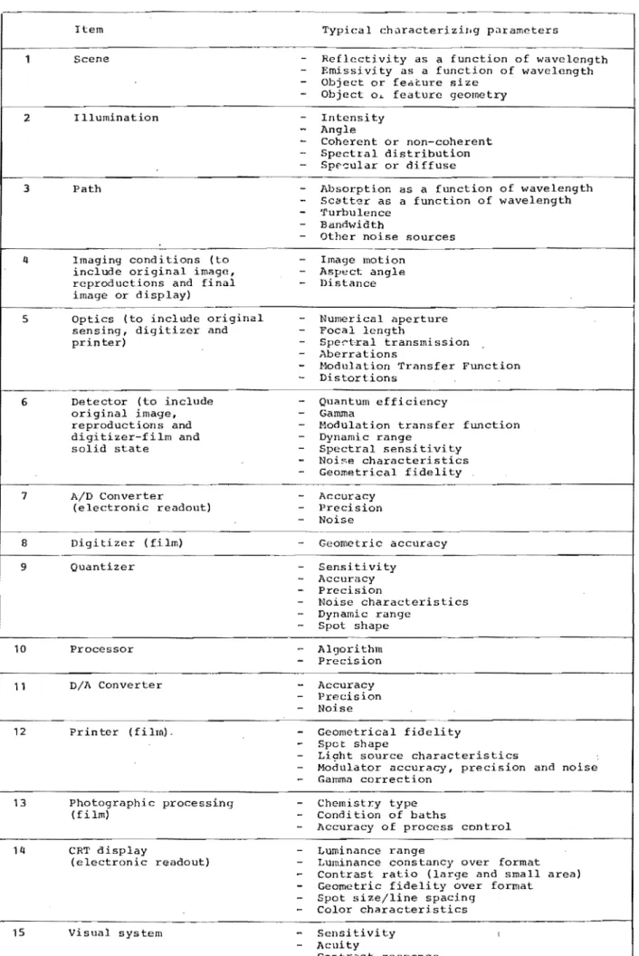
A methodology for the analysis of the imaging problem in general is known as image chain analysis (Booth and

Schroeder 1977). Figure 1.2 shows a number of the items which should be considered in analyzing the image chain. Each are components of the three major blocks identified above. The following sections deal with each of the three major blocks and analyze the components within the blocks.

1.2 IMAGE CONVERSION SYSTEM

The two-dimensional distribution of intensities over an object must be converted to a digital representation before i t can be processed by a digital computer. The

intensity of the image is detected by a sensor, or an array of sensors, to give an appropriate analog signal. This signal may either be an electrical signal or the exposure of a photographic film. The detection process requires that the two-dimensional distribution be spatially quantized into picture elements, or pixels. In addition to the spatial quantization, the intensity is also quantized when the

analog signal produced by the detector(s) is converted to a digital value.

--Item Typical chi1racterizing pi1rameters

1 Scene

-

Reflccti vi ty as a fUnction of wavelength

- Emissivity as a function of wavelength - Object or feature size

- Object 0 ... feature geometry

,---2 Illumination

-

Intensity

-

Angle

-

Coherent or non-coherent

-

Spectral distribution - Spf'-::ular or diffuse

- -

-~-3 Path - Absorption as a function of wavelength

-

Scatt'2!r as a function of wavelength

-

Turbulence

-

Bandwidth

-

other noise sources

4 Imaging conditions (to

-

Image motion include original image, - Aspect angle rcprod uctions and final

-

Distance image or display)

.~ ... ~~--.----~~~~-~--....

5 Optics (to include original - Numerical aperture sensing, digitizer and

-

Focal length

printer) - Sper'tral transmission

Aberrations

-

Modulation Transfer Function

-

Distortions

6 Detector (to include

-

Quantum efficiency original image, - Gamma

reproductions and - Modulation transfer function digitizer-film and

-

Dynamic range

solid state

-

Spectral sensitivity

-

Noige characteristics

-

Geometrical fidelity

7 A/D Converter - Accuracy

(e lectronic readout) - Precision - Noise

~~-~--- ---~--... ---~----...

-8 Digitizer ( film) Geometric accuracy

9 Quantizer Sensitivity

-

Accuracy

-

Precision

- Noise characteristics

-

Dynamic range

-

Spot shape

10 Processor Algorithm

-

Precision

c·_"

---11 D/A Converter

-

Accuracy

-

Precision

- Noise

. _ _ .... .

12 Printer (film) .

-

Geometrical fideH ty

-

Spot shape

-

Licht source characteristics

-

Modulator accuracy, precision and noise

-

Gamma correction

13 Photographic processing - Chemistry type

(film) - Condition of baths

-

Accuracy of process control

14 CRT display

-

Luminance range

(electronic readout) Luminance constancy over format

-

Contrast ratio (large and small area)

-

Geometric fidelity over format

- Spot size/line spacing

-

Color characteristics

15 Visual system

-

sensitivity ,

- Acuity

Contrast response Pattern recognition Color response

must be matched to the conditions established by the scene (1), illumination (2), path (3) and imaging conditions (4). For example, in remote sensing for land use classification, the reflectivity of the target vegetation in the near

infrared band (800-1100 nanometers) is important in determining the health of the vegetation (Bauer 1976). Therefore the sensor chosen must be sensitive to radiation in this band. The detector is also dependent on the level of the illumination. In very low light level applications, such as in surveillance work or in astronomical imaging, the sensor must have high quantum efficiency. The type of optics used in the imaging system depends to a large

extent on the physical attributes of the imaging situation. The aperture determines the intensity of illumination 'seen' by the detector and can be adjusted for differing conditions. The focal length determines the field of view and ground

resolution of each pixel. Recently, a spy satellite was reported to have a camera with a six metre focal length lens which could resolve whether or not a person on the ground was wearing civilian or military clothes (Richardson 1978) In the Landsat III remote sensing satellite, a ground coverage of 79 metres square for each picture element is achieved (Bauer 1976). The remote sensing system described in §2.3.1 was required to have a field of view of 0.35° so that when flying at an altitude of 6400 metres the

ground coverage would be 30 metres square for each picture element. This system requires a 6.4 mm focal length lens.

aberrations and distortions which produce geometrical

defects in the image (Thomas 1973; Jenkins and White 1976). Lenses also act as band pass filters. Normal glass lenses, for example, cut off the radiation in the infrared and

ultraviolet but quartz lenses have an enhanced response in the infrared relative to glass lenses.

1.2.1 Image Formation

The term image has been used loosely in the previous sections to describe a two-dimensional radiant field which is detected by a sensor and converted to a digital

representation by an analog-to-digital process. However, as castleman (1979) points out, the dictionary definition of an image is " ... a representation, likeness, or imitation of an object or thing . . . " Henceforth, the term image refers to the reproduction of the object's two-dimensional radiant fie ld.

Following Dainty and Shaw (§6.2, 1974) the formation of an image can be represented as in Figure 1.3.

n

Object Plane

/

/

/

/ . •

}---Imaging System

y

Image Plane

Figure 1.3 Image formation model.

For any general system, and for any input f{s,n), the output g (x,y) is

g(x,y) == S{f(s,n)}, (1.2-1)

where S{ • } is an operator acting on the input to produce the output. When the system is linear, an assumption which is realistic for many practical systems, the principle of superposition holds. That is, for all inputs f

1(s,n) and f ₂(s,n) and for all constants a and b,

S{af₁ (s,n) + bf₂(s,n)} = a S{f₁ (s,n)} + b S{f₂(s,n)}.

(1.2-2) Using the shifting properties of a delta function, any input can be considered to be a linear combination of weighted and displaced delta functions,

+00

f(s,n) ==

II

_{f(S1,n1) o(s - S1) o(n -n1)d s1 dn 1·} (1.2-3) - <X)

The output of the system is therefore, +00

g(x,y) =

S{I

I

f(S1 ,n

1) 0 (x - S1) 0 (y n1) d s1 dn 1 } (1.2-4) _ <X)

When f(s1,n1) is considered to be a weighting function

applied to the delta functions, the linearity property shown in equation (1.2-2) can be applied to bring the operator S within the integral

+00

g(x,y)

=

II

_{f(S1,n 1)S{o(x-r;1)o(y- 1)}ds1 dn 1 .} (1.2-5)

The response of the system at output coordinates (x,y) to a delta function at input coordinates (r;1,n

1) is defined as

The output of the system is then +00

g(x,y}

=

II

f(s,n}h(x,Yis,n)dsdn, (1.2-7) _ 00

where the subscripts have been dropped.

The system response to a delta function, equation (1.2-6), is called the point spread function (psf). In general, a point in the object plane does not image to a point in the image plane. The imaging system 'spreads' the point according to the psf. If the psf has the same shape over the image, i.e. i t depends only on the difference

between the variables and not on each variable independently, i t is a spatially invariant point spread function (sipsf). When this is the case,

h(X,Yis,n) = h(x - SlY n), (1. 8)

and

+00

g(x,y)

=

II

f(s,n) h(x-s,y-n)dsdn (1.2-9)

This is a convolution relationship and shows that the psf of the system must be spatially invariant for deconvolution image processing techniques to be effective.

An alternative term to describe the above condition is isoplanatism. The so called 'isoplanatic patch' is used in astronomical imaging to specify the viewing angle over which the psf is spatially invariant (see §4.1.1).

1.2.2 Image Characterization

measurable physical properties. An arraY~Qf detectors

measures an electromagnetic flux which, when integrated over time, gives the intensity distribution of the object. A number of attributes can be used to describe the physical measurements.

(a) ctral characteristics. The radiation received at the detector may be reflected by the scene

(reflectivity as a function of wavelength) or may be generated within the scene (emissivity as a function of

wavelength). The spectral characteristics give the relative radiant intensity of the object as a function of wavelength.

(b) Intensity. The detectors measure the radiation from the spatial distribution of image intensities. The intensity of a point in the image results in a flux field at the light sensitive surface of the detector. The dimensions of intensities may be given in radiometric terms, watts/ steradian, or in photometric terms, lumens/steradian (Spiro 1974) .

(c) Contrast. A measure which relates the range of intensities over the scene is the contrast. Booth and

Schroeder (1977) give several methods for calculating contrast.

Contrast as modulation:

==

=

=

(1.2-10)

Contrast for dark targets (L

t < Lb) 2 C

m

1 + C_m

where

Contrast for light targets (L

t > Lb) : 2 C

m

:=:

Contrast ratio:

Delta density: 1

+

C

L\D :=: _log10 m 1

-

C_m

L_t

=

target luminance Lb ::::: background luminance

L1

=

maximum luminance L2 = minimum luminance LO ::;:; average luminance ₌

(L 1

+

L₂)/2

(1.2-12)

(1.2-13)

(1. 14)

(d) Dynamic Range. The ratio of intensities of the brightest part to the dimmest part can characterized by the dynamic range. Dynamic range is usually defined as a

logarithmic expression,

Dynamic range

=

_{10 log10} (1.2-15)

where L1 and L2 are the maximum and minimum luminances in the scene.

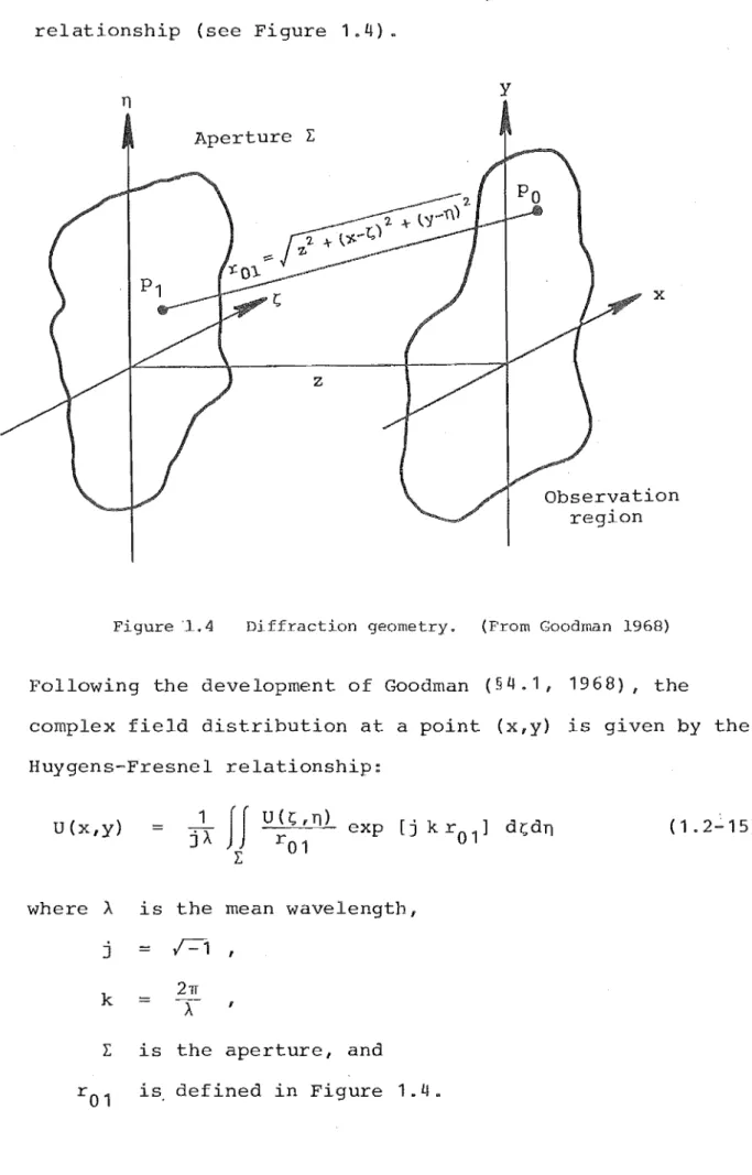
(e) Spatial frequency content. The concept of

in an aperture plane (~,n) is given by a Fourier transform relationship (see Figure 1.4).

n

Aperture E

z

y

x

Observation region

Figure '1.4 Diffraction geometry. (From Goodman 1968)

Following the development of Goodman (§4.1, 1968), the

complex ld distribution at a point (x,y) is given by the Huygens-Fresnel relationship:

U(x,y) 1

II

U(~,n) [j kr

01] d~dn (1.2":'15)

=

jA r exp

01 E

where A is the mean wavelength,

j :::::

F1

k

_T

21T

,

E is the aperture, and r

The integral can be written with infinite limits on the assumption that

U(s,n)

is zero outside the aperture

E.

I t is further assumed that the distance between the aperture and the observation plane, z, is much greater than any linear dimension in either the aperture or the

observation plane. These assumptions allow the sUbstitution of z for r

01 in the denominator of equation (1.2-15). The Fresnel approximation for r

01 uses the first two terms of a binomial expansion of the square root giving

=

(1.2-16)

The Fresnel approximation allows equation (1.2-15) to be written

U(x,y) = exp [j k z]

j A z

00

Jf

Expanding the quadratic terms in the exponent yields 00

U(x,y)

[ ' k

=

e xp [j k z] e xp

~

z

- 0 0

[ ' k

exp

~

z (

(1.2-17)

( 1 .2-18)

The Fraunhofer assumption applies for the far field where

Therefore in' the region of Fraunhofer diffraction

U(x,y} == exp[j k z]

j A z [

. k

exp

~

z (x2 +y2)]

II

u(r;,n)

-ex:>

exp [ - 21Tj

(A~

r; +

tz

nJ] dr; dn. ( 1 • 2- 2 0)

Except for the multiplicative factors preceding the integral which represent phase and magnitude scaling factors due to the geometry, the expression is a simple Fourier transform of the aperture distribution evaluated at frequencies

u == x z Therefore we can write

ex:>

v

=

l

AZ

u ( x , y)

=

K

I I

u ( r; , n) e xp [- 2 1T j (u r;

+

vn) ] d r; d n

where K is a complex constant.

(1.2-21)

(1.2-22)

As Shaw (1978) points out in his review of image evaluation methods, Luneberg (1944) and Duffieux (1946) showed the full advantages and implications of Fourier methods in optical image evaluation. A major advantage is that convolutions such as equation (1.2-9) I can be

transformed to become multiplications. This means that transfer functions for different components of the imaging system can be multiplied together to find the overall

transfer function algebraically instead of solving multiple convolution integral equations.

1.2.3 Image Detectors

Many textbooks explain the physics of the photoelectric effect (Holton and Roller 1958; Biberman and Nudelman 1971; Weidner and Sells 1975), and the characteristics of film

(photochemistry) have been well described by many authors (Thompson 1966; Brown 1966; Thomas 1973; Dainty and Shaw 1 9 7 4; Shaw 1 97 8) .

Solid state detectors are the prime interest here. Although photoelectric effect and photoemissive cathode devices are well understood and many devices are in use, e.g. television vidicon tubes (Chien and Snyder 1975), solid state sensors are becoming widely available and are suitable for many digital image processing applications. They can be made smaller and more robust because they do not require a vacuum or high accelerating voltages to operate. Fabricated with semiconductor technology, they can be mass produced and so are potentially less expensive than photocathode devices.

There are a number of important characteristics of solid state imaging devices.

(a) Quantum efficiency. In a photoelectric device, a photon is absorbed into the material of the device and an electron or a hole-electron pair is generated. These

function of wavelength for several photoelectric devices. (b) Sensitivity. The sensitivity of a solid state imaging array is defined as the minimum input flux which gives a detectable output. Sensitivity is therefore related to the noise performance and the responsivity or gain of the detector. Manufacturers such as Fairchild (1976) and

Reticon (1977) usually give the responsivity, which gives the output signal (volts per microjoules per cm2) and the

saturation exposure (microjoules per cm2

) . The spectral

energy of the input flux must be known before a calculation can be made to find the sensitivity of the device (see

§3.3.2) .

(c) Spectal response. Figure 1.5 shows the quantum efficiency of a device as a function of wavelength of the incident radiation This variability is known as the spectral responsivity.

_ 80 C

>-u

z

G

60

ii:

LL

lIJ

20

1000

Cs I (WINDOWLESS)

1500 2000 3000 4000 WAVELENGTH (l!.)

6000 8000 10000 ,

(d) Noise. There are many noise mechanisms which operate in photoelectric devices. Among these are photon noise, shot noise and thermal noise (Dainty and Shaw 1974; Chien and Snyder 1975; Billingsley 1975). In addition, dark signal and fixed pattern noise act to obscure the

desired signal. Taking into account all sources, the total noise can be considered to have two components,

= V

rms + VN (1.2-23)

where V_T is the total noise voltage, V is the rms value rms

and V

N is the fluctuating noise voltage.

( e) Dark signal. The dark signal is the component of the output signal which is not generated by incident radiation or by any readout process. The dark signal is measured in the absence of input radiation, hence its name. It is generally thermally generated and is a strong function of temperature, doubling every 7°C (Amelio and Dyck 1975; Murphy 1977).

(f) Fixed pattern noise. Fixed pattern noise is relevant in array sensors and describes the fixed nature of defective picture elements (Amelio and Dyck 1975). In

arrays such as the charge coupled device (see Chapter 3) elements can be defective by having too low or too high sensitivity. These are detected when the device is

illuminated with a flat field and remain constant in space and relatively constant in time (Murphy 1979).

attributable to capacitive effects but also include the trapping of charge carriers in surface energy states for later release into other signal charge packets.

(h) Qynamic range. The dynamic range of a device is defined as the ratio of the output signal when an input causes saturation to the output signal with no input

radiation. The dynamic range is expressed as a ratio or in decibles,

Dynamic range

=

V SAT 20 10910 V

rms

(1.2-24)

where V_SAT is the saturated output voltage and V

rms is the signal voltage output when no input is applied. It can be seen that the dynamic range is related to the average noise performance of the device.

(i) S

--~---al-to-noise ratio. The noise performance

of different devices is usually compared by the signa to-noise ratio, which gives, for a fixed iUwnination, the signal available compared to all sources of fZuctuating noise, V

N. The signal-to-noise ratio can be expressed in decibles,

SNR

=

V s 20 10910

V-N

where Vs and V

N are the signal and noise voltages.

(1.2-25)

g

₌

dR

dQ (1.2-26)

For any mean square fluctuation in the output ~R , the mean square fluctuation at the input required to produce ~R2 is

~Q 2 o

~R2

g2 (1.2-27)

DQE is defined as the ratio of actual mean square input fluctuation ~Q2 to the mean square output

referred to the input ~Q 2

o '

DQE

₌

uctuation

(1.2-28)

If Poisson statistics are assumed for the input quanta,

~Q2 = Q (1.2-29)

and

DQE

=

~

(1.2-30)

~R 2

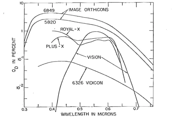
For detectors where the signal-to-noise ratio is quantum limited, Dainty and Shaw (1974) show that DQE may be expressed as,

DQE

=

(Output SNR) 2 (Input SNR) 2

(1.2-31)

where (Output SNR) is the signal-to-noise ratio at the output of the detector and (Input SNR) is the

10,.----,--!z

lLJ o II: lLJ 0..

10.1

Z

o o

0.3 0.5 0.6

WAVELENGTH IN MICRONS

Figure 1.6 Detective quantum efficiency Q

D for various detectors.

(From Jones 1957)

(k) Gamma. This term originally referred to the transfer characteristic of photographic 1m but is now used to define the characteristics of other transducers, e.g. CRT displays. In the photographic context, Figure 1.7 shows a curve of density as a function of log exposure. This

curve is known as the H-D curve after Hurter and Driffield. Three regions are shown on the curve. The low density/ minimum exposure horizontal portion is called the gross fog level (Goodman, §7.2, 1968). The central portion shows the linear relationship between density and log exposure, and the maximum density/maximum exposure region is called the solarization region (Shore 1974). The slope of the middle portion of the curve is called the gamma, y, and is defined

{l.Dp

y

₌

Gamma is a function of the type of film, exposure time,

and the type ~nd method of development.

2.0 ~huulu('r

Figure 1.7

(1) Linearity.

The Hurter-Driffie1d Curve. (From Goodman 1968)

Linearity is a term more often

app ed to photoelectric sensors than gamma. Linearity

expresses the deviation away from a 1:1 relationship between

the change in input radiation and the corresponding change

in output signal. Manufacturers commonly define linearity

as the maximum deviation from linear as a percentage of the

full scale output value.

(m) Geometrical effects. The geometry of an imaging

device specifies the accuracy with which the sensor records

the spatial distribution of the two-dimensional image

intensity. Geometrical effects include the fixed pattern

introduced by the lens, and non-linear scanning mechanisms in scannlng type sensors (Van Wie and stein 1977).

(n) Modulation trans function.

---~---- The modulation

transfer function (MTF) expresses the relative sensitivity of the device to spatial frequencies.

Following Dainty and Shaw (§6.2, 1974), consider a one-dimensional nusoidal input distribution,

f(x)

=

a + b cos (2nwx + £) (1.2-33) as shown in Figure 1.8 where w is the one-dimensional

spatial frequency and £ is a measure of phase.

Figure 1.8 Sinusoidal input distribution.

(From Dainty and Shaw 1974)

The input modulation is defined f

max f

max

- f . mln

+

f .

mln

=

b

The convolution relationship of equation (1.2-9) for the

output of an imaging system can be written

00

g(x,y)

=

If

f(x-z;;, y-n) h(Z;;,n) dZ;; dn

_.00 00

=

II

{a + b cos[2nw(x-z;;) + E]}h(z;;,n)dZ;; dn

- 0 0

(1.2-35)

where h(Z;;,n) is the spatially invariant psf. Integrating

with respect to n gives

00

g(x)

=

I

{a+b cos[2nw(x-z;;) +£]}l(Z;;)dZ;; (1.2-36)

_00

where 1(Z;;) is the line spread function. Using the expansion

of cos (A-B) and normalizing the spread function such that

its area is unity, equation (1.2 36) can be written as

g(x) ::: a+b cos(2nwx+£)

I

1(Z;;) cos 2nwz;; dZ;;

where

- 0 0 00

+ b sin(2nwx + E)

J

1(Z;;) sin 2nZ;; dZ;;

_00

a + b cos (2nwx + £)

c

(w) + b sin (2nwx + £) S (w)

C(w) - jS(w) == T(w)

=

J

1(z;;)exp(-2n j wZ;;)dZ;;

_00

(1.2-37)

(1.2-38)

The function T(w) is called the optical transfer function

(otf) and is the Fourier transform of the line spread

function. The modulus M(w) and the phase, ¢(w), of the otf

Nw) _tan

-1 (-S

_{C (w)} (w) ) (1.2-39)

and therefore

C (w)

=

M ( w ) co s 4l ( w)

S (w)

= -

M{w) sin /P(w) (1.2-40)

Equation (1. 37) can be written

g(x) == a+M(w) bcos(2TIwx+£+¢(w» (1.2-41)

Equation (1.2-41) shows that the output signal g(x) for a sinusoidal input is a sinusoid of the same frequency. The output modulation is defined

M

out

=

M(w)

b

a (1.2-42)

Thus the ratio of output modulation to input modulation is equal to the modulus of the Fourier transform of the line spread function, M(w).

In the more general.case for two dimensions, the MTF of the system can be shown to be the modulus of the Fourier transform of the point spread function.

These attributes relate to the characterizing of image devices and are valid for the evaluation of any image sensor. Solid state imaging arrays, such as charge coupled devices, are being used in many new applications where

1.2.4 Analog-to-digital Conversion

The imaging detectors convert radiation received from the source into an analog signal. The information must now be quantized and converted to a digital

representation. If film is the conversion medium, the film transparency is scanned with a digitizer which

measures the density of the film. This device is called a densitometer. See Shore (1974), Marcil (1974), and Dainty and Shaw (1974) for a review of densitometer techniques and instruments.

t Digital

npu Signal

-"c SIGNAL

CONDITIONING SamplQ

Start Convrzrt

Figure 1. 9

ANALOG SAMPLE

AND TO

HOLD DIGITAL

t

CONVERTER

Analog-to-digital conversion.

Data

End of Convarsion

The analog-to-digital conversion process used with photo-electrical devices is shown in Figure 1.9. The input signal from the sensor is first processed by a conditioning element. This provides buffering and isolation, amplifies the signal, and converts the polarity to that required by the sample-and-hold unit. The signal conditioning element also

sampling frequency, aliasing occurs in the output data (Shannon 1963).

To specify an analog-to-digital converter for use in an imaging system, a number of operating parameters must be considered. Among these are:

(a) Accuracy. Absolute accuracy of a converter should not be confused with the specification of linearity or resolution. Absolute accuracy is affected by three types of errors. These are the inherent

±!

least signi cant bit

(LSB) digital error, analog errors due to circuit tolerances, and aperture error. Aperture error results from uncertainty in the input voltage during the conversion time. (See

aperture time.) Relative accuracy is synonomous with

linearity, and specifies the deviation in the output codes from a straight line drawn through zero and full scale. Accuracy specifications are given in the number of bits deviation, usually least significant bit.

(b) Aperture time. This is the interval between the initiation of the conversion process, or a sample in the case of a sample-and-hold, and the output of the digital code. The aperture time determines the maximum error when sampling the analog voltage. For a signal of frequency f

M,

with a maximum amplitude V

M, and with an aperture time of tAP' the uncertainty in the input voltage ~V can be shown to be

(1.2-41)

By choosing a n bit converter and setting the ratio ~V/VM

with a maximum frequency component of fM and with an error of 1 LSB is

1 _(1.2-42)

=

(c) Conversion time. This is the total time

required to complete a conversion, and generally establishes the upper frequency limit of a signal which can be converted without aliasing.

(d) Resolution. The smallest analog input voltage for which the converter will produce an output code is the resolution. For example, an eight bit converter has a

resolution of 1 part in 256, or about 0.4% of the full scale value. Resolution and accuracy are often used interchange-ably in data sheets, but in the strict sense, accuracy refers to the measured deviation from the straight line performance over the entire range of the operation of the converter and resolution refers to the smallest signal which can be digitized.

(e) S

--~~---le-and-hold. Often, the aperture time

required to reduce the uncertainty in the input voltage to less than one least significant bit is far less than the conversion time required to satisfy the sampling rate from Shannon's theorem. When this is true, a sample-and-hold is used to sample the analog data and to hold i t at a constant value for the analog-to-digital converter during the

conversion time.

of the analog-to-digital converter. For example, a

resolution of 1 part in 1000 requires a 10 bit converter (n 10). If the upper frequency component in the input signal is 1 MHz, the conversion time, given by Shannon's theorem, must be at .1~'i()st 0.5 microseconds and the aperture time must be 0.16 nanoseconds. In this case, a sample-and-hold with an aperture time of less than 0.16 ns and a 10 bit converter with a 2 MHz data rate would be specified.

In practice, AID conversion systems have a number of other limitations. Departures from the ideal character-istics are defined by a number of secondary parameters including code skipping, gain accuracy, monotonicity, and slew rate. Useful references are Hnatek (1976) and Zuch

(1979) .

1 .3 DIGITAL PROCESSING SYSTEM

The previous section describes the analysis of the input conversion system and considers the image attributes, the sensor characteristics, and the conversion from analog to digital information. This section now considers the digital image processing but is restricted to reviewing the

analysis of image processing procedures in general. The

reason for this is twofold. First, many excellent reviews of image processing procedures have been published (Stockham 1972; Andrews 1974; Huang 1975; McDonnell 1975; Andrews

1977; Andrews and Hunt 1977; Castleman 1979). Secondly, a digital image processing procedure can be analyzed to determine whether or not i t is suitable for use in an

this suitability can be expressed in terms of the time which an operator can wait for results and still be effective in processing images or solving problems. Therefore, we need not consider the many image processing algorithms in detail other than to specify their operating characteristics.

1.3.1 Image Processin9 Characterization

The analysis of the processing step in interactive image processing systems considers the effect of the

processing on the image. The processor box (10) of Figure 1.2 indicates that the algorithm and the accuracy of the process must be considered.

(a) Algorithm. An important prerequisite for the development of an effective algorithm is a complete

understanding of the problem to be solved. This helps ensure that the algorithm will perform as required and not produce unwanted results. Program design techniques such as top down design and structured programming (Ledgard 1975; McGowan and Kelly 1975) emphasize problem analysis and design before writing programs. Producing efficient

algorithms, as Bentley (1979) points out, requires an insight into the wayan algorithm works. Hopcroft (1974) and Weide (1977) survey methods of evaluating algorithms, and Knuth (1968, 1969, 1973) provides examples of many

different algorithms. Unconventional approaches can produce highly efficient algorithm implementations. The 'brute

force and ignorance' method can also be interminable. Bentley (1979) cites the example of a sorting problem

algorithm and 4 seconds when a hashing technique 1S used. In image processing applications, the use of

look-up tables can significantly reduce the execution time of programs. However, one must balance the time required to calculate the index into the table, against the time to calculate the value itself. In assembler language

programming, the use of in-line code (macros) instead of subroutine calls can speed up the operation. This also increases the size of the program but as Brooks (1975) points out, there is a memory space-time trade-off which is valid over a remarkably wide range. In general, for a given function, the larger the program, the faster i t executes. An analysis of the accuracy with which

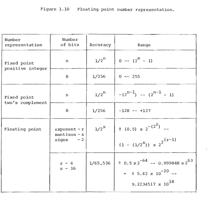
calculations are made can sometimes lead to a significant increase in the execution speed. Integer arithmetic is faster than floating point arithmetic when performed in software, and so changing from a floating point mathematics package to an integer package will allow the program to operate faster.

(b) Accuracy. The computational accuracy affects not only the final representation of the image but the processing itse , because a requirement for high