Do Macroeconomic Indicators Stimulate FDI Inflows in India?

(1)

ISSN Online: 2162-2086 ISSN Print: 2162-2078

DOI: 10.4236/tel.2017.77144 Dec. 12, 2017 2123 Theoretical Economics Letters

Do Macroeconomic Indicators Stimulate

FDI Inflows in India?

M. C. Minimol

Department of Business Administration, Rajagiri College of Social Sciences (Autonomous), Kochi, India

Abstract

The current study mainly attempts to find out whether macroeconomic indi-cators actually stimulate the inflow of FDI into India. The study also at-tempted to check whether there is any long run or short run relationship be-tween the macroeconomic indicators and FDI inflows into the country using regression analysis, Cointegration test, Granger causality and Vector error correction model. The results show that the explanatory variables captured in the model well explained the variations in FDI Inflows. However, not all the explanatory variables considered in the model are statistically significant in explaining the behavior of FDI. Unrestricted Cointegration Trace statistic and Max-Eigen statistics supports the existence of cointegrating relationship among the variables. The study also shows that SENSEX and NIFTY do gran-ger cause FDI in the long run while, FDI does not grangran-ger cause neither of the two. S Vector Error Correction Model supports the absence of short-run rela-tionship among the macroeconomic indicators and FDI inflows in India.

Keywords

Foreign Direct Investment, Sensex, Nifty, Gross Domestic Product

1. Introduction

The Foreign Direct Investment (FDI) is emerging as one of the most vibrant sectors witnessing remarkable growth in the 21st_{century. In the current global}

scenario, conditions favor both the host country and the investor, as Foreign Direct Investment (FDI) is any long term investment by an entity who resides outside the host country. It is not just an initial investment but a continuous process involving the need to keep investing looking at the needs and demands of the host country. Efficiency of the investment would be beneficial if the in-vestor factors in several local conditions like cheaper resources, bureaucratic

How to cite this paper: Minimol, M.C. (2017) Do Macroeconomic Indicators Sti-mulate FDI Inflows in India? Theoretical Economics Letters, 7, 2123-2133.

https://doi.org/10.4236/tel.2017.77144

Received: October 18, 2017 Accepted: December 9, 2017 Published: December 12, 2017

(2)

DOI: 10.4236/tel.2017.77144 2124 Theoretical Economics Letters

administration and tapping of talent specific to the host country. The payback in this kind of dynamic relationship is immense resulting in mutual benefits for both the investor as well as the host country. Transfer of technical knowledge, creation of a competitive market for the domestic industry, paving the way for other industries to invest and above all enriching the profit making ability of the investor in another country apart from his own are some of the reasons that has seen exponential growth in FDI.

This is especially true when it comes to India’s growth graph in FDI. It is an established fact that Foreign Direct Investment in any developing or under de-veloped country can play a crucial role in the growth of its economy; as there is a gap in the available resources and required resources. It is believed that FDI can fill this gap by driving required resources and know-how. This know-how trans-fer augments professional skills, reinforces infrastructure, guarantees the reach of international brands at doorstep, improves standard of living and generates employment opportunity. FDI is also viewed as a radical tool in accomplishing self-sufficiency of the economy in general. Considering its massive size of mar-ket, sound economic policies and abundant and skilled human resources, India has always been an alluring destination for international investors. Foreign di-rect investment in a country is the lone and most suitable tool integrating inter-national economy into a country’s economy. FDI helps in the balanced growth of the nation, maintenance of favourable BOP position etc. [1]

The structure of this paper is as follows. Section 2 addresses the relevant lite-rature and the objective of the study. Section 3 shows the model and empirical evidence drawn from the regression, cointegration tests, Granger causality tests and VECM estimations. Conclusions are provided in Section 4.

2. Review of Literature

Bhattacharya and Satinder [2] in their study Foreign Direct Investment in India: Facts and Issues attempted to study the new economic reforms which contri-butes technological up gradation, level of production and access to the global market and critically analyzed the FDI regulations of the country. Study focused on the various aspect of Foreign Direct Investment in India. Singh and Singh [3], analysed the trend of FDI inflow to India, during the period 1970-2007 using time series data.

(3)

considerable collision on export concert even though the FDI has a favorable correlation. Chen [5] brought out a study on the Location Determinants of For-eign Direct Investment in Developing Countries and concluded that countries which dissuaded foreign investment inflows received only very less FDI com-pared to other countries with higher per capita income, bigger market size and faster economic growth that encouraged foreign investment. Kumar and Kar-thika [6] pointed out in their study sectoral performance through inflows of for-eign direct investment, that the host country is benefitted in the field of eco-nomic development due to foreign direct investment.

Foreign investment and modern technology has aided to boost the pace of economic growth in most of the host countries. Foreign Direct Investment at-tracts large inflows of capital knowledge and technological resources into the economy of the country.

Using a process structure, this paper studies Foreign Direct Investment inflow into India and stake of top ten investing countries flow into India. Dikhit and Shringarpure [7] studied the role of Foreign Direct Investment on economic growth in India. Anitha [8] tried to study the elements determining the inflow of foreign investment and the reasons for lesser inflows and their corrective ac-tions.

The paper share the common view that foreign direct investment plays a vital role in the economic progress of any developing country; the reason being the gap of required funds/resources and available funds/resources. The develop-ments and anticipated foreign direct investment for a period of five years are summarized in the study using Autoregressive Integrated Moving Average (ARIMA) technique. The study identifies skilled human resources, huge market size, stable economic structure and ample natural resources as the factors con-tributing to attract FDI and ascertains lack of political determination, insuffi-cient infrastructure and lack of storage facilities as the causes for less inflow of FDI.

(4)

of foreign direct investment in Indian Economy by finding out the relationship between Foreign Direct Investment and the macro economic factors like GDP, Inflation and NIFTY movements.

Almost all the studies done on foreign direct investment are focusing either on the trend and nature of the foreign direct investment or how it affects the economic growth of the host country. There exist gaps in the literature, regard-ing the determinants of FDI inflows to a host country.

Majority of econometric theory is built up on the assumption of stationarity. The presence of a unit root in the series indicates that the time series is not sta-tionary but that differencing will reduce it to stasta-tionary. Augmented Dickey [13]

Fuller test is a test for unit roots which is based on an approximation of an auto regressive-moving average model by an autoregression. Stationarity tests allow verifying whether a series is stationary or not. There are two different approach-es: stationarity tests such as the KPSS test that consider as null hypothesis Ho that the series is stationary, and unit root tests, such as the Dickey-Fuller test and its augmented version, the augmented Dickey-Fuller test (ADF), or the Phil-lips-Perron test (PP), for which the null hypothesis is on the contrary that the series possesses a unit root and hence is not stationary. The present study is based on unit root tests. Regressing a non-stationary variable Y up on a non-stationary variable x, may lead to a spurious regression, in which estimators and test statistics are misleading. The use of non-stationary variables does not neces-sarily result in invalid estimators, especially the two variables are cointegrated,

i.e., if there exists a particular linear combination of these non-stationary riables that is stationary. In such cases, a long run relationship between these va-riables exist. The existence of such long run relationship also has its implications for the short run behaviour of the variables because there has to be some me-chanism that drives the variables to their long run equilibrium relationship. This mechanism is modelled by an error correction mechanism, in which the equili-brium error also drives the short run dynamics of the series [14].

Johansen maximum likelihood cointegration test establishes [15] [16] the long-run relationships among the variables being investigated. In examining causality, the Granger causality analysis was performed.

However, Johansen co-integration test does not indicate anything about the direction of causality among the variables in the system; therefore, the Granger causality analysis was done. If the series are co-integrated, the VECM-based Granger causality analysis is an appropriate technique used to determine the long-run and the short-run relationships [17]. The Granger representation theorem [18] states that if a set of variables are cointegrated, then there exists a valid error correction representation of the data.

(5)

rela-DOI: 10.4236/tel.2017.77144 2127 Theoretical Economics Letters

tionship between them.

3. The Model and Empirical Evidence

The current study is an attempt to highlight the role of macroeconomic variables in stimulating FDI inflows in India. Much of the literatures in economics and finance support the ability of macroeconomic indicators to stimulate growth in the ecomomy, especially in developing countries. Existing theoretical evidence largely suggests that macroeconomic variables can predict the flow of foreign investment to a country. Thus the present study considers eight commonly used macro-economic variables including Balance of Payment (BOP), Consumer Price Index (CPI), Exchange Rate (ER), SENSEX, NIFTY, Foreign Exchange Re-serve (FER), Gross Domestic Product (GDP) and Gross National Income (GNI) as the predictors and FDI inflows to India as the dependent variable for empiri-cal testing and model building. The entire study is conducted with the help of E Views 8 software. Data relating to each variable from 1970-71 to 2015-16 were collected from various bulletins of Reserve Bank of India.

To avoid the problem of spurious regression that often occurs from non-stationarity of time series data, the unit root tests were carried out on all the data of the variables considered in the model. The unit root test was performed using Augmented Dickey-Fuller (ADF) and Philip Peron (PP) test. To test the hypo-thesis that there is unit root.

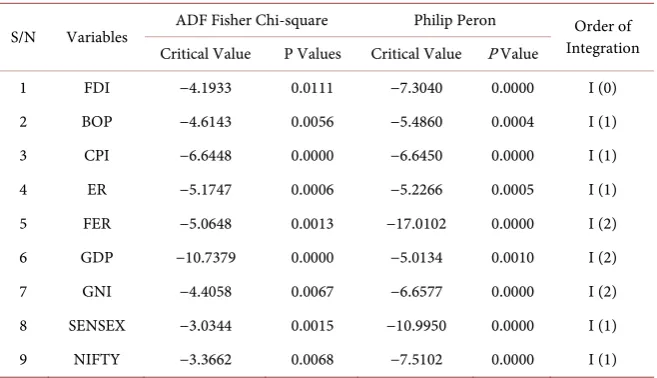
The results of unit root test and Philip Peron (PP) test are presented in Table 1.

[image:5.595.211.540.520.709.2]

Reading from Table 1 above and applying the decision rule, we can conclude that FDI, BOP, CPI, ER, SENSEX, and NIFTY are stationary at first order of in-tegration while FER, GDP and GNI are stationary at second order of inin-tegration. Hence, the time series of these variables are deem fit to be used for estimating regression model at the order of integration for which they are stationary.

Table 1. Results of unit root test and Philip Peron (PP) test.

S/N Variables ADF Fisher Chi-square Philip Peron _IntegrationOrder of Critical Value P Values Critical Value P Value

1 FDI −4.1933 0.0111 −7.3040 0.0000 I (0)

2 BOP −4.6143 0.0056 −5.4860 0.0004 I (1)

3 CPI −6.6448 0.0000 −6.6450 0.0000 I (1)

4 ER −5.1747 0.0006 −5.2266 0.0005 I (1)

5 FER −5.0648 0.0013 −17.0102 0.0000 I (2)

6 GDP −10.7379 0.0000 −5.0134 0.0010 I (2)

7 GNI −4.4058 0.0067 −6.6577 0.0000 I (2)

8 SENSEX −3.0344 0.0015 −10.9950 0.0000 I (1)

9 NIFTY −3.3662 0.0068 −7.5102 0.0000 I (1)

(6)

Having conducted stationarity test for all the time series data and then consi-dered it to be appropriate for regression analysis at their differences, the result of regression model is presented below:

0 1 2 3 4 5

6 7 8

FDI BOP CPI ER FER GDP

GNI SENSEX NIFTY it

β β β β β β

β β β µ

= + + + + +

+ + + + (1)

FDI 1074.74 0.2679BOP 0.0676CPI 443.03ER 0.0686FER

0.2262GDP 0.1926GNI 2.8310SENSEX 18.244NIFTY

= + − − −

− + − +

Std Error: 1483.73 0.2007 3.2394 476.70 0.0622 0.4449 1.1169 5.7974

T. statistic: 0.7243 1.3347 −0.0209 −0.9294 −1.1019 −0.5084 0.4449 −2.5346 3.1470

P-value: 0.4817 0.2049 0.9837 0.3696 0.2905 0.6197 0.6637 0.0249 0.0077

R-squared: 0.8367, Adjusted R-squared: 0.7362, F-statistic: 8.32, P-value: 0.0004, Durbin Watson: 1.97

The results of FDI regression model estimated shows that FDI would be 1074.74 when all the independent variables modelled are assumed to be zero. It is paramount to note that of all the 8 explanatory variables only 3 variables (BOP, GNI and NIFTY) have positive relationship with FDI while the rest have negative relationship with FDI. This translates to: a 1% increase in BOP, holding the other variables constant, will increase FDI by 26.79% and vice versa. One per cent increase or decrease in GNI and NIFTY, while other variables presumed to be constant will result in 22.62 per cent and 182.44 per cent increase or decrease in FDI in that order. As appeared in the model estimate that CPI, ER, GDP and SENSEX have negative relationship with FDI—a 1% increase in CPI, ER, FER, GDP and SENSEX will cause FDI to decrease by 6.76%, 44.03%, 06.86%, 22.62% and 28.10% respectively.

The regression result can be trusted and be relied upon for analysis and pre-diction as most of the economic expectations are met. The model shows that the explanatory variables captured in the model explained 83.67% of the variations as R2_{is 0.8367 and}_R2_{adjusted is 73.62% which suggests that after penalized}

those variables and factors that do not really influence the behavior of FDI, R2

adjusted still exhibit that independent variables account for 73.62% changes in model. However, not all the explanatory variables considered in the model that are statistically significant in explaining the behavior of FDI even though they may influence it positively and negatively by the nature of their relationship with it. The estimate shows that only SENSEX and NIFTY have significant impact on FDI; SENSEX has negative and NIFTY has positive relative with it. This is evi-dent as the probability values of t-statistics of each associated variable is less than 5% and the standard errors of each statistically significant variable are less than half the parameters of the associated variable.

(7)

implies that our estimation does not suffer from serial correlation and auto cor-relation. As such, the model is statistically reliable in explaining the relationship between FDI and its determinants.

3.1. Johansen Cointegration Test

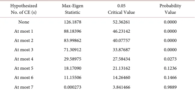
Having estimated regression model, Johansen Cointegration was conducted to decide if there is any long run relationship among the variables considered. Un-restricted Cointegration Trace statistic and Max-Eigen statistic are established to determine whether cointegration exists.

The results are given in Table 2 and Table 3.

[image:7.595.210.539.343.509.2]

The Johansen tests are called the maximum eigenvalue test and the trace test. For both test statistics, the initial Johansen test is a test of the null hypothesis of no cointegration against the alternative of cointegration. The tests differ in terms of the alternative hypothesis. The maximum eigenvalue test examines whether the largest eigenvalue is zero relative to the alternative that the next largest ei-genvalue is zero. If the rank of the matrix is zero, the largest eiei-genvalue is zero,

Table 2. Unrestricted cointegration rank test (Trace).

Hypothesized

No. of CE (s) Statistic Trace Critical Value 0.05 Value P

None 428.5955 159.5297 0.0000

At most 1 302.4077 125.6154 0.0000

At most 2 214.2237 95.75366 0.0000

At most 3 130.2251 69.81889 0.0000

At most 4 58.91598 47.85613 0.0033

At most 5 29.32623 29.79707 0.0566

At most 6 11.15533 15.49471 0.2021

At most 7 0.000273 3.841466 0.9889

Source: Johansen Cointegration Test, Eviews 8.

Table 3. Unrestricted cointegration rank test (maximum eigenvalue).

Hypothesized

No. of CE (s) Max-Eigen Statistic Critical Value 0.05 Probability Value

None 126.1878 52.36261 0.0000

At most 1 88.18396 46.23142 0.0000

At most 2 83.99862 40.07757 0.0000

At most 3 71.30912 33.87687 0.0000

At most 4 29.58975 27.58434 0.0273

At most 5 18.17090 21.13162 0.1236

At most 6 11.15506 14.26460 0.1466

At most 7 0.000273 3.841466 0.9889

[image:7.595.211.539.554.709.2]

(8)

there is no cointegration and tests are done. If the largest eigenvalue λ1 is

non-zero, the rank of the matrix is at least one and there might be more cointegrating vectors. The trace test is a test whether the rank of the matrix Π is r0. The null

hypothesis is that rank (Π) = r0. The alternative hypothesis is that r0 < rank (Π) ≤

n, where n is the maximum number of possible cointegrating vectors. Both un-restricted Cointegration Trace statistic and Max-Eigen statistics supports the ex-istence of cointegrating relationship among the variables in the study.

3.2. Granger Causality Test

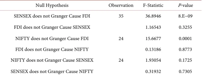
This statistic is normally adopted to discern whether a particular variable will be better explained and predicted by having another variable as its determinant other than itself. In Pairwise Granger causality test, F-statistics and its associated p values are used to determine whether one factor has long-run effect on another variable (i.e., by incorporating one variable into another would help in explain-ing the variation in variable in the long run). From Table 4, two independent variable which were found to be statistically significant are considered together with FDI and six scenario of Granger causality tests are depicted. We accept the alternative hypothesis for the four scenario and reject the null hypothesis for two scenario. The table shows that SENSEX and NIFTY do granger cause FDI in the long run while, FDI does not granger cause neither of the two. In addendum to that, NIFTY does not granger cause SENSEX and SENSEX does not granger cause NIFTY. By granger cause, we imply that NIFTY and SENSEX do have long run effect on FDI.

3.3. Vector Error Correction Model

Since that two methods of Cointegration (Johansen Cointegration and Granger causality test) show that the independent variables employed have long-run ef-fect on the dependent variable, the Vector Error Correction model was adopted to investigate whether there would be short-run deviation from the long run ef-fect.

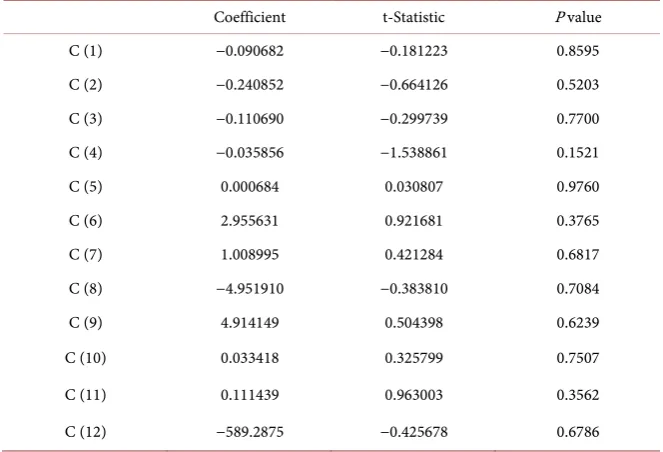
[image:8.595.211.541.585.711.2]

Table 5 and Table 6 show the result of Vector Error Mechanism (VECM) which were computed to investigate whether there is short-run disequilibrium in

Table 4. Pairwise Granger causality tests.

Null Hypothesis Observation F-Statistic P-value SENSEX does not Granger Cause FDI 35 36.8946 8.E−09 FDI does not Granger Cause SENSEX 1.16543 0.3255 NIFTY does not Granger Cause FDI 24 15.6677 0.0001 FDI does not Granger Cause NIFTY 0.13186 0.8773 NIFTY does not Granger Cause SENSEX 24 1.93054 0.1725 SENSEX does not Granger Cause NIFTY 0.31932 0.7305

(9)

[image:9.595.210.539.88.361.2]

DOI: 10.4236/tel.2017.77144 2131 Theoretical Economics Letters Table 5. Vector error correction model 1.

Error Correction: D (FDI) D (GDP) D (SENSEX) D (NIFTY) D (FER) Coint Equation (1) −0.090682 −17.25145 −0.695982 −0.102232 −7.991217

[image:9.595.208.540.408.634.2]

(0.50039) (6.42117) (0.25722) (0.06037) (2.23226) [−0.18122] [−2.68665] [−2.70575] [−1.69353] [−3.57988] D (FDI(−1)) −0.240852 18.75446 0.969069 0.179131 9.921206

(0.36266) (4.65378) (0.18642) (0.04375) (1.61784) [−0.66413] [4.02994] [5.19820] [4.09435] [6.13237] D (FDI(−2)) −0.110690 15.26814 0.063997 0.011251 0.847555 (0.36929) (4.73886) (0.18983) (0.04455) (1.64742) [−0.29974] [3.22190] [0.33712] [0.25254] [0.51448] D (GDP(−1)) −0.035856 1.244052 0.014577 0.003082 0.185073 (0.02330) (0.29900) (0.01198) (0.00281) (0.10394) [−1.53886] [4.16071] [1.21702] [1.09638] [1.78050] D (GDP(−2)) 0.000684 0.428654 0.032087 0.005923 0.190215 (0.02221) (0.28500) (0.01142) (0.00268) (0.09908) [0.03081] [1.50406] [2.81054] [2.21074] [1.91988]

Source: VECM, Eviews 8.

Table 6. Vector error correction model 2.

Coefficient t-Statistic P value

C (1) −0.090682 −0.181223 0.8595

C (2) −0.240852 −0.664126 0.5203

C (3) −0.110690 −0.299739 0.7700

C (4) −0.035856 −1.538861 0.1521

C (5) 0.000684 0.030807 0.9760

C (6) 2.955631 0.921681 0.3765

C (7) 1.008995 0.421284 0.6817

C (8) −4.951910 −0.383810 0.7084

C (9) 4.914149 0.504398 0.6239

C (10) 0.033418 0.325799 0.7507

C (11) 0.111439 0.963003 0.3562

C (12) −589.2875 −0.425678 0.6786

Source: VECM, Eviews 8.

(10)

Reading from Table 6, it is glaring that coefficient and t-statistic of C (1) are negative but they are not statistically significant on account of its associated probability value that is more than 5 per cent. In Table 6, no coefficient has probability value of 0.05 or less, this implies there is no short-run relationship among the variables used in the model.

As seen from the results, FDI inflows to India, Balance of of Payment, Con-sumer Price Index, Exchange Rate, Sensitivity index, and NIFTY are stationary at first order of integration while Foreign Exchange Reserve, Gross Domestic Product and Gross National Income are stationary at second order of integra-tion. Hence, the time series of these variables are deem fit to be used for esti-mating regression model. The regression model shows that the explanatory riables captured in the model well explained the variations in the dependent va-riable. Both unrestricted cointegration Trace statistic and Max-Eigen statistics supports the existence of cointegrating relationship among the variables in the study. SENSEX and NIFTY do granger cause FDI in the long run while, FDI does not granger cause neither of the two. It is also revealed that, NIFTY does not granger cause SENSEX and SENSEX does not granger cause NIFTY. VECM proved that there is no short-run relationship among the variables used in the model.

4. Conclusion

(11)

References

[1] Jasbir, S., Sumita, C. and Anupama, S. (2012) Role of Foreign Direct Investment in India: An Analytical Study. Research Inventy: International Journal of Engineering and Science, 1, 34-42.

[2] Bhattacharya, B. and Satinder, P. (1996) Foreign Direct Investment in India: Facts and Issues. Indian Institute of Foreign Trade, Occasional Paper, 1-19.

[3] Singh, S. and Singh, M. (2011) Trends and Prospects of FDI in India. Economic Af-fairs, 56.

[4] Kishor, S. (2000) Export Growth in India: Has FDI Played a Role? Center Discus-sion Paper No. 816, Economic Growth Center, Yale University.

http://ageconsearch.umn.edu/bitstream/28372/1/dp000816.pdf

[5] Chen, C. (1997) The Location Determinants of Foreign Direct Investment in De-veloping Countries. Working Paper, Chinese Economic Research Centre, University of Adelaide. Australia.

[6] Kumar, G.L. and Karthika, S. (2010) Sectoral Performance Through Inflows of For-eign Direct Investment. https://ssrn.com/abstract=1705946

[7] Dikhit, S.V. and Shringarpure, A.A. (2014) The Role of Foreign Direct Investment on Economic Growth in India. Asian Journal of Management Sciences, 2, 120-122. [8] Anitha, R. (2012) Foreign Direct Investment and Economic Growth in India.

Inter-national Journal of Marketing, Financial Services & Management Research, 1, 108-125.

[9] Lodhi, G.S. (2014) Foreign Direct Investment in India: A Critical Analysis on FDI.

International Journal of Core Engineering & Management, 1.

[10] Priya, D. and Jyoti, B. (2013) Impact of FDI Inflow on Service Sector in India: An Empirical Analysis. International Journal of Management Research and Business Strategy, 2, 120-129.

[11] Park, J. (2004) Korean Perspective on FDI in India. Economic and Political Weekly, 31 July 2004, 3551-3555.

[12] Prabhakaran, V. (2015) Role of Foreign Direct Investment in Indian Economy.

EPRA International Journal of Economic and Business Review,3, 139-145. [13] Dickey, D.A. and Fuller, W.A. (1979) Distribution of the Estimators for

Autoregres-sive Time Series with a Unit Root. Journal of American Statistical Association, 74, 427-431.

[14] Enders, W. (2004) Applied Econometric Time Series. John Wiley and Sons, New York.

[15] Johansen, S. (1988) Statistical Analysis of Cointegrating Vectors. Journal of Eco-nomic Dynamics and Control, 12, 231-254.

https://doi.org/10.1016/0165-1889(88)90041-3

[16] Johansen, S. (1991) Estimation and Hypothesis Testing of Cointegration Vectors in Gaussian Vector Autoregressive Models. Econometrica, 59, 1551-1580.

https://doi.org/10.2307/2938278

[17] Engle, R.F. and Granger, C.W.J. (1987) Co-Integration and Error Correction: Re-presentation, Estimation, and Testing. Econometrica, 55, 251-276.

https://doi.org/10.2307/1913236

[18] Granger, C.W.J. and Weiss, A.A. (1983) Time Series Analysis of Error-Correcting Models. In: Karlin, S., Amemiya, T. and Goodman, L.A., Eds., Studies in Econome-trics, Time Series, and Multivariate Statistics, Academic Press, New York, 255-278.