Visualizing differentials in integration to picture the fundamental theorem of calculus

University of Warwick institutional repository: http://go.warwick.ac.uk/wrap This paper is made available online in accordance with

publisher policies. Please scroll down to view the document itself. Please refer to the repository record for this item and our policy information available from the repository home page for further information.

To see the final version of this paper please visit the publisher’s website. Access to the published version may require a subscription.

Author(s): David Tall

Article Title: Visualizing Differentials in Integration to Picture the Fundamental Theorem of Calculus

Published in Mathematics Teaching, 137, 29–32 (1991)

Visualizing Differentials in Integration

to Picture the Fundamental Theorem of Calculus

David Tall

Mathematics Education Research Centre University of Warwick

COVENTRY CV4 7AL

Introduction

What is a differential? From my investigations asking sixth-formers arriving at university about concepts in the calculus, the evidence shows a manifest confusion in

the meaning of notations such as _{dx and} dy ∫ f(x) dx. Many students repeat the received

wisdom that _{dx means the derivative of a function y=f(x) and should be thought of as}dy

a single indivisible symbol, not as a quotient. Those who do give dx a meaning as a separate entity invariably talk of a “very tiny change in x” or an “infinitely small change in x” or even “the limit of δx as it tends to zero”. Meanwhile the dx in ∫ f(x) dx means

“with respect to x”, though students need to be willing to make the substitution

du = du_{dx dx , to compute the integral by substitution. A little later they may be faced}

with the problem to solve the differential equation

dy dx = –

x y

(where they had been told that dy_{dx is an indivisible symbol) by “separating the}

variables” to get

y dy = – x dx

(what does the dx mean here?) then put an integral sign in front to get

∫ y dy = – ∫ x dx

(where presumably dx now means “with respect to x”), to obtain the solution(s)

y2

2 = –

x2

2 + c.

us a passport to become fully fledged members. I confess that, along with most of my colleagues, I learned to cope with the routines and got the right answers until I ceased to ask awkward questions about the meanings of the symbolism.

A perusal of calculus textbooks in current use shows some very neat ways of sidestepping the fundamental issues of meaning, but few seem to have a totally coherent view of the meaning of differential that works throughout the calculus.

In an earlier article1 I discussed the visual interpretation of the differential in differentiation, but at the time had not yet appreciated a possible analogous use of the differential dx in the integral ∫ f(x) dx.

In this article I will show that there is indeed a simple meaning that can be given to dx which works in both differentiation and integration – a meaning that was given by Leibniz in his first publications on the calculus2,3

– a meaning that takes on a new and vigorous life in our modern computer age. For three hundred years Leibniz has been maligned in the English-speaking world, first as a man who stole Newton’s theory of the calculus, and then as someone who invented an incredibly useful but curiously mystical notation. He deserves better treatment. All it requires is to look at the right pictures.

1. The differential in differentiation

This is an easy matter to explain and has been well represented in the literature (see, for example, Quadling4). The derivative of a function f at a point x is found by calculating

f(x+h)–f(x)

h

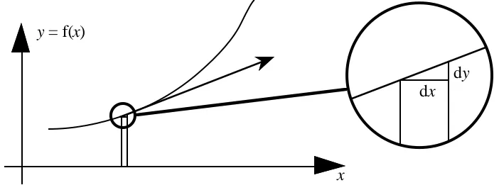
and considering what happens as h gets small. If it tends to a limiting value, this is denoted by f'(x) and called the derivative of f at x. It is, of course, the gradient of the tangent to the graph at x. If dx is any real number, then dy is defined as

dy = f'(x) dx.

3 -dx

dy = f'(x) dx

y = f(x)

x

figure 1: dx and dy as components of the tangent vector

Computer graphics now help us visualize that, under high magnification, a suitably small portion of the graph of a differentiable function will look straight. Thus, when dx is suitably small, then dy is a good approximation to f(x+dx)–f(x) (figure 2).

dx dy

y = f(x)

x

figure 2: magnifying a locally straight portion of the graph of a differentiable function

This insight will prove valuable in linking this use of the differential with that in integration.

2. The differential in integration

Let us begin by attempting to give the differential in integration the same meaning as in

differentiation: dx represents a change in x. We will use the notation Σb

x=a f(x) dx or Σ b a

f(x) dx to denote the sum of the areas of strips width dx, height f(x) between x=a and

x=b. (In Britain, the more usual symbol is Σb

x=a f(x) δx, where δx denotes a small

3. Visualizing the Fundamental Theorem

y=f(x)

x

dx f(x)

a b

figure 3 : The area sum Σba f(x) dx

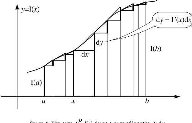
To understand the relationship between the use of dx here and that in differentiation, all we have to do is to look at the right picture. Figure 3, which for so long has been the standard view is not the right one for the fundamental theorem. We must look not at the graph of y=f(x), but at the graph of y=I(x) where I'(x)=f(x). We will assume for the moment that such a function I can be found, returning to the conditions under which it exists in the next section. Given such an I where I'(x)=f(x) we simply draw the corresponding picture for y=I(x) with the same subdivision of the interval [a,b] into sub-intervals (figure 3).

y=I(x)

dx dy

I(b)

I(a)

a x b

dy = I’(x)dx

figure 4: The sum Σb_a f(x) dx as a sum of lengths Σ dy

At each point x of the subdivision we draw the tangent to the curve I(x), then the corresponding increment to the tangent is

5

-Thus the sum Σba f(x) dx is seen as the sum of the lengths Σ dy where each dy is the

vertical component of the tangent vector to the graph of y=I(x). The sum Σ dy is the sum of the vertical line segments, and, provided that the dx are taken to be small so that the graph is relatively straight from x to x+dx, then this is approximately equal to the increment to the graph, I(x+dx)–I(x). Adding together the increments to the graph from

x=a to x=b simply gives I(b)–I(a). Thus adding together the vertical steps dy may in

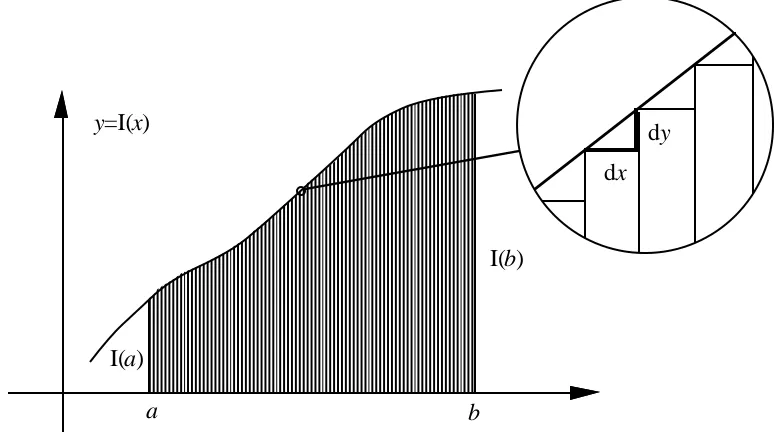
some sense approximate to I(b)–I(a). Figure 4 gives a fair indication of this idea. It fails in part because we had to make the strips fairly wide to see what is going on and this, in turn, means that the graph may be so curved in a strip that dy is clearly different from I(x+dx)–I(x). But imagine it instead as having a large number of strips, and imagine a part of the graph being magnified to see its local straightness with a few strips next to each other (figure 5).

b y=I(x)

a

I(a)

I(b)

dy dx

figure 5: looking closely at the summation process

Now it should be possible to imagine that as the lengths dx get smaller, the sum of the lengths Σdy approximates to I(b)–I(a).

The picture only gives a sense of what is going on. But the zooming-in process should hint at something more. As one zooms in, the curved graph gets less curved. Students who use a graph-plotting program readily appreciate this phenomenon. It was the first thing that the first students to play with Graphic Calculus observed without any prompting.

and the actual step to the curve gets less. In this way we get a hint that the errors are now small in proportion to the vertical step, so adding them together, the total error is also now small in proportion to the total vertical step. In other words we may begin to see that, as the lengths dx get smaller, the sum of the vertical steps, Σdy, gets closer to I(b)–I(a).

The symbol ∫ba f(x) dx is used to represent the limit of Σ b

a f(x) dx as (the maximum

size of) dx gets small. The argument just given provides a powerful intuition as to why this limit is likely to be:

∫ba f(x) dx = I(b)–I(a).

4. Proving the Fundamental Theorem

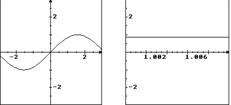
Although we may now have a sense of why the fundamental theorem of calculus might be true, this does not yet constitute a proof. For instance, what are the conditions on the function f which would guarantee that there is a function I such that I' = f ? Until we can establish this we cannot even draw figures 4 and 5, because we cannot be sure of the existence of the function I. I have earlier shown how one might visualize the likely properties required of f by looking at the graph of f in a different way6,7. I suggest that interesting pictures might occur by maintaining a constant y-range whilst taking a much smaller x-range. For instance, figure 6 shows the graph of y=sinx with the same

y-range in each (–3 to 3) but x-range being changed from –3 to 3 down to 1 to 1.01.

What happens is that the graph in the second case is pulled flat by the stretching of a thin x-range to fill the computer window.

Figure 6 : The graph of y=sinx, pulled out flat

7 -A(x+h)–A(x) ≈ f(x)h.

This suggests that we may have

A(x+h)–A(x)

h ≈ f(x),

and perhaps, as h → 0, we might get

A'(x)=f(x).

What kind of function, when stretched out horizontally near x=x0, looks flat ? If we

suppose this means that the graph lies in a pixel representing a height f(x)±ε, then we need to know that, given such an ε > 0, then we can find a small enough x interval, say

x±δ, so that when t lies between x–δ and x+δ, then f(t) lies between f(x)–ε and f(x)+ε. In other words, a natural condition for the function to satisfy the fundamental theorem is that it be continuous in the formal sense:

Given any ε>0, a δ>0 can be found such that whenever x–δ < t <x+δ we know that f(x)–ε < f(t) < f(x)+ε.

For such a function if the width of a strip h is taken positive and less than δ then the value of f(t) will lie between f(x)–ε and f(x)+ε throughout the strip and so

(f(x)–ε)h < A(x+h)–A(x) < (f(x)+ε)h.

Hence

A(x+h)–A(x)

h

is sandwiched between f(x)–ε and f(x)+ε. A similar argument holds for h negative. As

ε is arbitrary, this is the formal definition that

lim

ε→0

A(x+h)–A(x)

h = f(x),

i.e. A'(x) = f(x).

Note that this only requires the continuity of f(x), not that it be differentiable. The reader who has completed a university mathematics degree will doubtless know this theorem. But can you see why it is true with your inner eye?

is exhibited by seeing that when magnifying the graph it never looks straight (figure 7) and continuity by stretching the graph horizontally to see it pull out flat (figure 8) 8,9

.

Figure 7 : The blancmange function being magnified near x=1/3

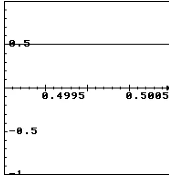
Figure 8 : The blancmange function being stretched horizontally from x=0.499 to x=0.501

9

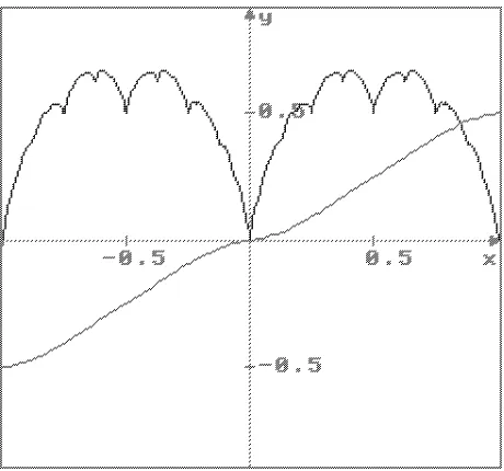
-Figure 8 : The area function for the blancmange and its (approximate) derivative

Using Real Functions and Graphs 10 _{on the Archimedes computer, it is possible to}

draw (a numerical approximation to) the area function for a(x), which is a graph b(x) whose derivative is a(x) and whose second derivative is the blancmange function. This builds an approximation to a graph which is everywhere differentiable twice, but nowhere three times, even though its second derivative is continuous. It is relatively boring to draw, yet illustrates the concept which is otherwise hard to imagine: the possibility of a graph differentiable twice but not three times, or, more generally, n times but not n+1 times.

References

1. Tall D. O. 1985: “Tangents and the Leibniz notation”, Mathematics Teaching, 112 48-52.

2. Leibniz G. W. 1684: “Nova methodus pro maximis et minimis, itemque

tangentibus, qua nec fractas, nec irrationales quantitates moratur, & sinulare pro illis calculi genus”, Acta Eruditorum 3, 467-473.

3. Leibniz G. W. 1686: “De geometria recondita et analysi indivisibilium atque infinitorum”, Acta Eruditorum 5.

4 . Quadling D.A. 1955: Mathematical Analysis, O.U.P., Oxford.

5. Woodhouse R. 1803: The Principles of Analytical Calculation, Cambridge.

6. Tall D. O. 1982: “The blancmange function, continuous everywhere but differentiable nowhere”, Mathematical Gazette, 66, 11-22.

7 .Tall D.O. 1986: Graphic Calculus II (for BBC, Nimbus, Archimedes computers), Glentop Press, London.

8. Tall D. O. 1986: Graphic Calculus I (for BBC, Nimbus, Archimedes computers), Glentop Press, London.

9. Tall D. O., Blokland P. & Kok D. 1990: A Graphic Approach to the Calculus, (for IBM compatibles) Sunburst, Pleasantville, NY.