Some energy related functionals and their vertical variational theory

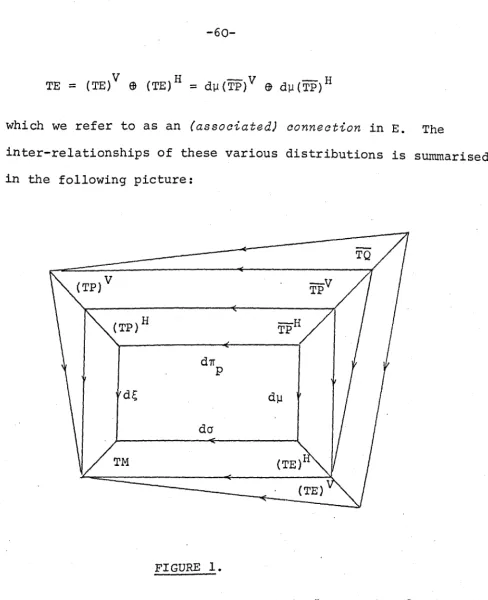
warwick.ac.uk/lib-publications

Permanent WRAP URL:

http://wrap.warwick.ac.uk/78846 Copyright and reuse:

This thesis is made available online and is protected by original copyright. Please scroll down to view the document itself.

Please refer to the repository record for this item for information to help you to cite it. Our policy information is available from the repository home page.

SOME ENERGY - RELATED YillIC,rIONALS , AND THEIR VERTICAL VARIATIONAL THEDRY

by

Christopher M. ~[ood

Thesis submitted for the degree of Doctor of Philosophy.

Mathematics Institute

University of Warwick

In memory of our brother, Tim.

" lord, you establish peace for me;

all that I have accomplished, you have: done for me."

ACICOt~LEDGEMENTS

I would like to express my deepest gratitude to my supervisor,

Professor Jim Eells, \"lhose powers of inspiration and encouragement were

at all times a sufficient catalyst for my researching and writing this

thesis.

My special thanks go also to my family for their constant sympathy and support, whilst at times wondering what on earth I was upto.

Of all my many contemporaries at the University of Warwick Maths

Institute, I would particularly like to th~~ Peter Hall, Howard Sealey,

and Michael Weiss, for the elucidation which, probably unbeknown to them,

they helped to provide.

I am grateful to the Science Research CounCil, as it was then known,

for financial support during the period 1978 - 1981 •

Illy final thanks go to Terri Moss for resolutely typing a manuscript which would have otherwise severely taxed the limited typographic skills

The energy and volume of a mapping of Riemannian manifolds are

linked by a discrete family of functionals, indexed by the elementary

symmetric polynomials. We explore the variational properties of members

of this family; in particular, their tension fields, stress-energy tensors,

~~d Jacobi operators.

When one Riemannian manifold fibres over another, applying the

conventional theory of harmonic maps to sections neglects the additional

structure supplied by the fibering. We give an alternative definition

for harmonicity of sections which overcomes this deficiency, and is

closely- enough linked to the conventional theory to share many of the

qualitative properties of harmonic maps. Such "harmonic sections"

arise as solutions to a variational problem, one consequence of which

is to allow the proof of a reduction theorem for harmonic sections of

a Riemannian vector bundle.

The "Gauss section" of an isometrically immersed submanifold

extends the idea of "Gauss map" to ambient spaces of arbitrary curvature.

We prove a non-trivial identity relating Gauss map to second fundamental

form, and generalize to the Gauss section. This leads to a

character-ization of immersions with harmonic Gauss section, and to a further

identity involving a suitably generalized notion of "third fundamental"

form". We are also able to characterize those Riemannian foliations of

(i)

INI'RODUCTION

Given an m-dimensional,. smooth, oriented. Riemannian manifold (H,g), a

symmetric function o:;JRm-lR, and a diagonalisable tensor field B on lit of type (1,1), we may form the O"-integral associated to B by evaluating 0 on

the spectrum of 3 and integrating over (M,g). This construction is

mentioned at the beginning of [E-SJ, where it is also !1oted that when

cp: (£f,g) - (W,h) : is a mapping of Riemannian

manifolds:-(i) The energy of cP is the Cj1/2 - integral,

(ii) The volume of cP is closely related to the Cjm-integral ,

where the or-integral in question is that associated to the (1,1) tensor

*

obtained (by "raising an index" ) from the pulled-back metric cP h , and the rth elementary symmetric polynomial (1r. Since then,R.Reilly has

worlced-out the variational theory for the (1 -integrals associated to the shape

r

operator of an immersed hypersurface ([Rei]), fundamental to the mechanics

of which are certain divergence-free Newton tensors. Inspired by his

exa~ple, and undeterred by the fact that the relevant Newton tensors are

no longer divergence-free, Chapter 1 of this.thesis attempts to do the

same for the fclJ"nily of energy-related (1r-integrals. We begin by laying

out with som~ care the tools of the variational trade - for these are to be redeployed in Chapter 3 where slightl~ more subtlety is involved -and proceed to investigate the critical points of ( j under variations of

r '.

the two independent para..lleters of map CP, and domain metric g. In analogy

wi th the theory for 0"1 ' we have called the corresponding Euler-Lagrange

operators higher-power tension fields, and stress-energy tensors,

respectively. ?ne qualitative picture is much as one would expect. Fbr

instance, on ascending the ladder (whose bottom and top rungs are the

energy and volume functionals respectively), the class of "trivially

higher rank. This is reflected in the quasi-linearity,of the

higher-power tension fields and Jacobi operators, with consequent complications

regarding their ellipticity. There is also a generalization to

even-dimensional manifolds of the conformal invariance and volume-majorizing

properties of the energy functional on maps of surfaces - a natural idea

here is that of r-conformalitl of a map, generalizing weak conformality.

On accolL~t of this, it is tempting to look for nice links between properties

of r-harmonic maps of 2r-manifolds, and the complex geometry of any

holo-morphic structures which may be imposable. HOwever, there is evidence to

suggest that the "bottom rung" may be somewhat special in this respect;

notably that, when r 1, any r-conformal, r-harmonic map of a 2r-manifold

is necessarily homothetic (or r-trivial

J (

Propositions 1.7.2 and 1 .1 .3 )

No such thing is true for weakly conformal harmonic maps of a surface, although in this case much is owed to the remarkable properties of

Riemann surfaces. We conclude Chapter 1 with a calculation of the

Euler-Lagrange equations for the volume functional, making .use of higher-power

stress-energy.

Chapter 2 is a catalogue of various results in the geometry of fibre

bundles, for later use, but recorded here to establish notation and

allow the expositions of later results to proceed unhindered. Sections 3

and 4

,

which are referred to in Chapter

_.

4, deal with the geometry of fibre products and endomorphism bundles, and are almost self-evident. So also

is our brief account of connections in vector bundles from the viewpoint

of connection maps ( §6

J,

which seems the most appropriate for the discussion of Chapter 3 §3. Section 2 is a useful decomposition result

for curves in a bundle with connection, and is the lynchpin for the proof

(iii)

results concerning Riemannian immersions and submersions. Besides being

of interest in itself, this result is used throughout the thesis.

The title of Chapter 3 is perhaps a little misleading, for the idea of

"harmonic sections it is to generalize the grap~ of a harmonic map rather than to look at bundle cross-sections which are. themselves har~onic maps.

Thus, we are interested not simply in sections "lhose tension field.,

vanishes, but those with vanishing vertical tension fie~~. In the first

instance, the generalization from graphs to sections of non-trivial fibre

bundles is made by looking at the associated .equivariant maps. We then

introduce the (higher-power) vertical energy functionals and examine their

variational theory. It is not surprising that the two notions of harmonic

section thus arising coincide. HOwever, it is interesting to note that

the apparently greater degPee of generality permitted by the variational

viewpoint (namely, loosening "fibre bundle" to any submersion of Riemannian manifolds ~ and "section" to any map) . cannot be fully allowed if there is

to be any hope of computing the Euler-Lagrange equations. Indeed, we are

tlforced" into considering the restricted variational problem of varying a

section through sections, and placing (fairly natural) geometrical

constraints on the submersion itself .

.

Having hitherto worked vIi th the entire range of energy-related

functionals, we now discard the higher-povler energies and look at the

1-harmonic sections of vector bundles. From the variational point of

view it is natural to consider Riemannian vector bundles (Lemma 3.3.3)

and compactly-supported sections (more generally, sections of finite;

vertical enert;!), in which case linearity permits the reduction of the

second order vertical tension field to a first order system. This is

seen as a generalization of the fact that every harmonic map of finite

Chapter by rephrasing for harmonic sections the existence and unique

continuation properties of harmonic maps.

In Chapter 4 we exploit the theory of harmonic sections to study the

geometry of isometrically immersed submanifolds. ~vhen the ambient

space is Euclidean, or more generally of constant curvature, it is

possible to define an associated Gauss map, which takes its values in

an appropriate Grassmannian. The geometry of the Gauss map is then •

nicely related to, the geometry of the immersion (cf

[a-v],

[C-G] , [Oba] ,

[Ish]). By replacing the Gauss map with the Gauss section (of the

appropriate Grassmann bundle), it is possible. to obtain a complete

generalization which places no restrictions on the ambient space, and

has correspondingly richer geometrical content. At the heart of the

matter is a connection-preserving vector bundle fibre isometry

(!)

which identifies the 2nd

f~damental

form of the immersion with the

vertical differential of its Gauss section (Proposition 4.2.4). Having

obtained this identity, we find ourselves on level ground. On one hand,

applying the Codazzi equation gives an instant generalization of the

theorem of Ruh-Vilms; ; 'on the other, after making a suitable definition

of the third fundamental form, an.~:.application of the Gauss equation gives

an identity of quadratic differentials extending that of M.Obata ( [R-VJ,

[Oba]). Through the consideration of a couple of examples, we are lead

to the idea of an Einsteinian immersion, in which case the generalized.

version of Ruh-Vilms theorem simplifies to a virtual facsimile of its

original. Being fulfilled whenever the ambient space has constant

curvature "Einsteinian" is also the extra condition required for the

,

theorems of Obata's paper to find their place in our more general setting

(Corollary 4.2.6 ).

(v)

of the case when the ambient space is Euclidean, for which we offer the

following three justifications. The first is simply to fill a gap in

the literature, previous expositions (e.g. [R-V] , [C-G] ) having omitted

to supply details of their implicit geometrical identifications ( see

Propositions 4.1.1 , 4.1.3, and 4.1.4 below). However, when the ambient

space is flat, it is in these very identifications that all the geometry

lies! Secondly, the properties of one of the identifications (Proposition

4.1.3 ) are needed to prove the "vertical part" of its subsequent

general-ization (Proposition 4.2.3). And thirdly, the proof of Proposition 4.2.4

is directly motivated by that of Proposition 4.1.4.

Our original motivation for a generalization of Ruh-Vilms' theorem

came from the study of the Gauss section of a Riemannian foliation - in

particular, the question "When is the Gauss section harmonic? II (following

a tentative conjecture

ap~earing

on the last page of [KT2] ) - and the

concluding section of Chapter 4 returns to this. Of course, the question

is well-posed for foliations of arbitrary codimension, but in choosing

to approach the problem by piecing together the Gauss sections of

individual leaves matters are considerably simplified in co dimension

_,

one. The basic reason for this is that a co dimension one Riemannian

foliation is invariant under parallel translation along normal geodesics,

with the consequence that there is no normal contribution to the vertical

tension field of the full GausS section. It also happens that in

codim~

ension one the generalized Ruh-Vil~s theorem also simplifies, so that

the final result (Theorem 4.3.1 ) is fairly succint. Even so, the explicit

appearance of curvature shows the conjecture of [KT2] to be rather over.

optimistic. As a particularly nice example, we cite the isoparametric

hypersurface foliation of a space form (after removing focal varieties),

Chapter 1 A FAMILY OF ENERGY FUNCTIONALS 2 3 4

5

6 7 8

Product manifolds

Induced vector bundles

Variations

Newton polynomials and Newton tensors

Higher - power energy

The first variation 0 f Er (cpt ,g) - tension fields

The second variation of Er (cpt ,g) - Jacobi operators

The first variation of Er (cp,~ ) - stres's-energy tensors

Chapter 2

1 Generalities

2 Horizontal! vertical decomposition of paths

3 Fibre products

4 Hom - bundles

5 Partial connections

6 Connection maps

Chapter 3 Il'AR.MJ NIC SECTro 1:5

1

2

3

4

Graphs of r-harmonic maps

Vertical energies

Harmonic sections of a Riemannian vector bundle

Existence and unique continuation of harmonic sections

Chapter 4 THE GAUSS SECTro N

1 The Ruh-Vilms theorem

2 The Gauss section of a Riemannian immersion

3 The Gauss section of a Riemannian foliation

NOTATION

For the most part, our notation agrees with that of

Kobayashi and Nomizu([K-N]), including their choice of sign

for the curvature tensor. Points at vlhich we may diverge are

usually due to the influence of Spivak ([Spi]); for example:

If a:E + M is a (smooth) fibre bundle, then the space of

(smooth) sections of a is denoted by teE).

Ifa:E + M is a vector bundle, with dual bundle a*:E* + M,

then we ai:>oreviate the tensor bundle E* €;) ••• €;) E* €;) E €;) ••• €I E + M

'"-.... _ - -... . . - - - ' # \.. • . /

to

~~(a) :'~(E)

+ M, and write teE)

when a =TM:TM + M,. we abbreviate

=

ij}

k,i=1

t~(TM)

to

k

.t

k

~ i (E) • In particular,

~~

(H) •

The Lie algebra of a Lie group is, on the whole, denoted

by the corresponding lower case Gothic character. For the

classical groups, this is only partially true; for example,

O(n) has Lie algebra a(n).

The summation convention is taken to be in force, unless

otherwise indicated.

As regards cross-referencing, each Remark, Lemma,

Proposition, Theorem and Corollar~r is numbered with respect to the section (§) in which it appears. If mentioned elsewhere

in the same chapter, this nUliwer is preceded by the relevant

section number; if referred to in another chapter, a further

§1. PRODUCT MANIFOLDS

Let TIp (resp. TI Q) denote the projection from the product P x Q of two smooth manifolds onto P (resp. Q), and, for each

(x,y) E P x Q, let

iy:P + P x Qi x ~ (x,y), jx: Q + P x Qi Y ~ (x,y)

be the corresponding inclusions. The tangent bundles

l' p: TP + P and 1'Q:TQ + Q may be "spread out" over P x Q by

defining vector bundles:

R

(x, y)

di (T" P) etc.

y x

,

-so that T(P x Q} is isomorphic to TP

e

TQ. Any vector field

on P (or Q) may then be extended to P x Qi for'example, if

X E t(TP}, define

X

E t(TP} by

X

o i

=

di

Y Y o X. A product

fieZd on P x Q is any of the form

X

+ Y, where X E t(TP} and

Y E t(TQ}; by writing (v,w) for di (v) _{Y , x} + dj (w) E T( _x,y } (P x Q)

(where v E TxP and w E TyQ) we have that

X

=

(X,O),

Y

=

(O,Y),

and

X

+

Y

=

(X,Y). Conversely, starting with a vector field

Z on P x Q and restricting to fibres of TIp (resp. TIQ) produces

a family of vector fields on P (resp. Q):

c t (TP) • "

Say that Z is Q-invariant if Z

=

Z for all y~ E Q. Product

Y1 Y2 ...

fields are clearly both p-invariant and Q-invariant - they are

-2-Through the existence of local product frame fields in

T(P x Q), product fields are sufficient to characterise

geometry in P x Q. Thus, if (P,k) and (Q,i) are Riemannian

manifolds, P x Q has the product metric:

k x i«X,Y), (X',Y'))

=

k(X,X') + i(Y,Y')

w.r.t. which TP and TQ are orthogonal, and each of rrp' rrQ

a Riemannian submersion. Also:

Proposition

The Levi-Civita connection for (p x Q, k x i) is

charact-erised by:

PXQ~ (X' Y')

=

(p~xX" Q~yY.') (X, Y) ,

for all X, X, E C(TP) and Y, Y' E C(TQ).

Proof. Such a connection in T(P x Q) is metric and

torsion-free. c

§2. INDUCED VECTOR BUNDLES

Let rr:E ~ N be a vector bundle, and ¢:P ~ N. Write

' f \ ,

¢-1 rr :¢-1 E ~ P for the vector bundle induced by ¢, and ¢ for

~-1E

=

{(p,e) E P x Ei TI(e)

=

~(p)}

IV

>

E

.

,

~(p,e)

=

e

In

P

>

N

Corresponding to any section a of TI is .the pullbaok seotion

-1 -1

~ a of ~ TI:

f -1 ~

Remark 1. I ~

=

TIp:P x Q -+ P, then TIp (TP) TP and

-1

TIp (X) ++ X for any X E t(TP).

Since pullback sections provide local fibre bases for

~-1TI'

they are sufficient to characterise geometry in

~-1E.

Thus, if TI has fibre metric g, $-1 TI has the pullbaok metrio

-1 ~ g:

1 -1 -1 (

<P~ g(~ a,~ 13)

=

g(a,I3), for a~l a, 13 E t E).

Similarly, if TI has connection V,

~-1TI

has the pullbaok

oonneotion ~-1V:

Remark 2. If (E,g,V) is a Riemannian vector bundle, so is

-1 -1 -1

(~ E,~ g,~ V).

A morphism TP

2->

E

..j- TI

N

-4-section of T*P

~

¢-1 E• The A-torsion of V (see [KT2] is

-I-P

-1

then that ¢ E-valued 2-form on P:

for all Z,Z' E C(TP). If D is any connection in TP, the

covariant derivative of A (tensor product connection) is

referred to (c.f. [ViI]) as the fundamentaZ form seA) of A

(w.r.t. D and V):

Proposition 1

TV,A(Z,Z')

=

seA) (Z',Z)-S(A) (Z,Z') + A(TD(Z,Z'»

Where TO is the usual torsion of D. In particular, if D is

torsion-free and A has symmetric fundamental form, then TV,A

=

O.

Proof.

=

SeA) (Z' ,Z) + A(DZZ') - seA) (Z,Z') - A(DZ'Z) - A[Z,Z']

=

seA) (Z',Z) - seA) (Z,Z') + A(TD(Z,Z'». o·

In anticipation of Chapter 3, §1, let ~:P + M, and

1jJ -1 (ni) ,II/!

_>

_TM ; I1jJ (p,v)

₌

di _(1jJ(p»(v) <j,(p)

.} .}

P

>

M x N

1jJ x ep

for any pEP and v E T1jJ(p)M.

Proposition 2.

(ii) If (M,g), (N,h) are Riemannian manifolds, then I1jJ and Iep

are connection-preserving fibre isometries.

Proof. Let X E C(TM} and Z E C(TP). We observe that:

(i) Firstly, I1jJ

°

d1jJ(Z) + Iep

°

dep(Z)

=

d1jJ(Z) + dep(Z)

=

(d1jJ(Z), dep(Z». Now, TIM

°

(1jJ x ep) _,

=

1jJ and TI _N

°

(1jJ x ep) = tf.,

't'

so that, for any pEP:

For any (x,y) E M x N, iy

°

TIM projects M x N onto M x {y},

so that d(iyOTIM) (x,y) is the projection of T(x,y) (M x' N) onto

TM(x,y) along TN(x,y)'

(ii) We show that I1jJ commutes with covariant differentiation

-6--1 I1jJ (V'z1jJ X)

=

-1

=

(1jJx¢) (V'd1jJ(Z)X,O), by Proposition 1.1.

§3. VARIATIONS

~ . l,;

Suppose initially that M ---) Q ---) N, and that E is a

vector bundle over N. Then (l,; o~) -1 E is isomorphic to

~-1l,;-1E,

an isomorphism being:

Il,;,~:(q,e) -+ (q,(~(q),e», for 1T(e)

=

l,; 0 ~(q).

Moreover, (l,; 0 ~)-1E and ~-1l,;-1E are geometrically

indist-inguisable:

Proposition 1

If E has a connection and fibre metric, then I ~ is a

l,;,<"

connection-preserving isometry.

Proof. We check that I ~ commutes with covariant

l,;,<"

differentiation as pullback sections. If a E teE) and

WEt (TQ) :

-1 -1 -1 -1 -1

V'W(Il,;,~(l,;o~) a)

=

V'w(~ l,; a)

=

~ (V'd~(W)(l,; a»

-1 -1 - 1 ·

=

~ l,; (V'dl,;od~ (W)a)

=

Il,;,~ «l,;0~) V'd (l,;o~) (W)a)

-1

=

Il,;,~(V'W(l,;o~) a)

where V' denotes the connection in E along with its various

pullbacks, as appropriate. CI

A variation of ¢:M -+ N is a smooth q,:M x JR -+ N with

q,(x,O)

=

¢(x) for all x E M. Then, replacing Q by M x JR gives the following example of the above:

y,~~l(TN)

I

i ~ 1 q,-1 (TN)· /~~_/_'V----> q, -1 (TN)

1 ,//

i t

1

-...,.'V-->

q,

TN

1

M

--->

M x JR

---->

N

By virtue of Proposition 1, we need make no further distinction

between

¢~1

(TN) . and

i~1q,-1

(TN). If ;t denotes the product

field (0,

d~)

on M x JR, define the variation fie Zd of q, by

a

-1

v = dcp 0 at E C (q, (TN) ); for each t E JR, . put

.-1 -1 -1

v t

=

~t v E C(¢t (TN». Conversely, any section

Vo

E t(¢ (TN» determines a variation ¢t(x)

=

exp t vO(x) (subject to a choice

of connection in TN) whose variation field agrees with

Vo

at

t

=

O.

Concerning variations of tensor fields on M, for each

,.

t E JR let it: ~ (M x JR) -+ ~(M) be the extension to ~(M x JR) of:

,.

t (T (M x JR) ) it(Z) = _{Zt' for all Z} E

'" _{i~n,for all n} E t (T* (M x JR» • it W) =

For any B E

C([~(M

x JR», _{let Bt}

=

itB E

C(l~(M»,

and define dB_t k

-8-Proposition 2

dB

tj

dt s 1/

. -a

a

t B .

Proof. We prove the case k = 2, i = O. If X,Y E C(TM), then:

Now,

Thus:

(1/

a

B)

<x,y)

=

at

1/

a

at

(B(X,y» ..:. B(I/

a

X,y)

at

A

a

--=

at B(X,Y) B(I/(O ~)(X,O),Y) 'dt

=

:t B(X,y), by Proposition 1.1.

B (di (X), di (Y» _{s s}

B(X,I/ (0 ~) (Y,O»

'dt

=

B(X,Y)oi • s

( is 1/

a

B) (X, Y)

=

(1/ a B) (X,

Y)

ois

=

a~

B (X,

Y)

ois at

at

=

l' _{~m -1 {B(X,y)} t-+O t

0

i s +t - B(X,y) 0 _is}

l' _{1 {B t(X,Y) - B (X,Y)}} dB

tl

=

~m - = dt s (X, y) • [J

t-+O t s+ s

If h is a Riemannian metric on N, and ~ a variation of ¢:M -+ N

with variation field v, then ~*h is a variation of ¢*h with

proposition 3

where

{Ei}~

is any local frame field in M with dual

{ei}~,

and Sym denotes "syrnrnetrisation".

Proof. By Proposition 2:

"

*

d¢thl =" is

dt s ¢*h

"

=

(i iJ s

a

at

i ¢*h)(E.,E.) e

~ J

(i iJ

s

a

¢*h)(E.,E.) ~ J

=

(iJ "I 0 ¢*h)(E.,E.)oi ~ J s

=

~t

• ¢*h(E.,E.)oi

ot: l. J S

at

at

by Proposition 1.1.

NOw, since (¢-1 (TN), ¢-1 h , ¢-1NiJ) is a Riemannian vector

bundle (Remark 2.2):

=

h(V

a

_{(d¢OEi),d¢(E j}

»

_{+ h(d¢(Ei ), iJ}

a

(d¢OEj»~

at

at

We note that d¢ has symmetric fundamental form ([ViI]'>, V is

torsion-free, and [E

i , :t]

=

0, so that by Proposition 2.1:

a

-_.¢*h(E.,E.)

at

~ J

a

-

-

a

=

h (iJ - (d¢ o,crt) ,d¢ (E.) ) +h (d¢ (E. ) , V_E- (d¢ 0 "ITt»

E. J ~.

-10-Now

d¢

(E . )

0 i = d¢ 0 di 0 E. = d<p (E.)

J s s J s J

and

v) _is -1 -1 'V_E v

('V- 0 = i ('V

E

v) = 'VE(i v) =

Ei s ~ . ~ . s ~ . s

,

so that:

o i = h('V

E v ,ei<p (E.» + h(d<P (E.) ''VE v ). s . s s J s ~ . s

~ J

o

Increasing the number of parameters in a variation gives

rise to higher order variation fields. In particular, if <P _s, t

is a 2-parameter variation of <P:M -+ (N,h) with variation fields

a¢ a¢ nd

v

=

as

and w

=

at' then the 2 order variation fields of ¢*h are given by:

Proposition 4.

at as

=

2 Sym {h"(RN(W,d<P(Ei»V + _{'VE. 'V a v,d<P(E}

j » ~

at

+ h('VE.v,'VE.w)}

e

i @

e

j •

~ J

(Omitting subscript (s,t) for notational clarity) •

Proof. (cf. [Smi] Proposition 1.1)

,..

=

i _s,t 'V.... 'V

"-a a

at

as

4l*h) (E.,E.)e i ® ej

~ J

=

(IJ

a

IJ

a

at

as

4l*h)

(E.,E.)

oi ei®ej

~ J s,t

=

IJ d [IJ d _{(4l*h(Ei ,Ej} »] 0 is,t e

i

® ej , by Proposition 1.1.

at

as

As in the proof of Proposition 3:

IJ "I (4l*h(E.,E.»

=

(J ~ J

as

so that

NOw,

and

h(IJE.v, d4l(E.» + h(d4l(E.),IJ

E- v),

~ J ~.

J

+ h(IJE.w,IJE.v) + _{h(d4l(E i} ),1J d IJE.v).

~ J

at

J

N

-R (w,d4l(E.»v

~

[

d~'

E

i ]

=

0, from which the result follows. c

§4. NEWTON POLYNOMIALS AND NEWTON TENSORS

-12-(J (x 1'···,x) l: ef" 7 0 "4 ,;> ~"

=

x. . .. x.

r m

i _1<···<ir ~1 ~ r

P (x₁'···,x)

=

xr r 1 +

...

+ xm

r m

f _r (x₁" " ' x ) _m

r

=

(_1)r l:

k=1 x. • •• x. ~1 ~k

(For example,

f1

=

_{x 1 '}

f2

=

x2 _{1 - x 2 '}

Lemma 1. ( [Wae] p. 8 1 )

Lemma 2.

=

f3 f4 r l: p=O

=

=

3 x 1 4 x 1 -2x

1x2 + x3

2

-

3x

1x2 + 2x₁x₃

x

r-p f _P

=

O.

2

+ x

2 - x 4 )·

[J

[J

Suppose B is a diagonalisable endomorphism of an

m-dimensional real vector space.Let (Jr(B) and Pr(B) denote

the corresponding polynomials in the eigenvalues of B, and

let fr (B)

=

fr (0'1 (B), ••• ,am (B».

In the polynomial ring

~[xJ,define

the rth Newton polynomial

of B by:

XB,r (x) = r

p () p .( r r r-1 r

r

(-1) 0r_p B x = -1) {x -01 (B)x + ... +(-1) Or (B)

p=O

~k 2. If XB(x) = det (xl -B), the characteristic polynomial

m

of B, then XB,m = (-1) _XB•

The Newton polynomials of B satisfy the following recurrence

relation:

Lemma 3.

XB,r (x) =Or (B) - x XB,r-1 (x) • o

We may use the fr(B) to "invert" the Newton polynomials:

Proposition 1.

r r

x

=

r

(-1)P f (B)X_B (x) =

=0 r-p ,p

r

(-1) {XB,r (x)

+ ••• -t

Proof. By induction on r.

Firstly, x = -(01 (B) - x) + 01 (B) = -XB,1 (x) -t f1 (B).

Now, by the induction hypothesis:

r+1

x _{= (-1)r{XX} r

B,r(x)-f1 (B)xXB,r-1 (x)+ ••• +(-1) fr(B)x}

= (_1)r+1{X (x)-f (B)X (x)+ ••• +(-1)rfr (B)XB 1(x)}

B,r+1 1 B,r ,

r + (_1)r{Or+1 (B)-f

1 (B)Or(B)+ ••• +(-1) f·r (B)01 (B)}, by Lemma 3.

By Lemma 2, the second summand is just fr+1 (B), which completes

-14-Since~r(B) is a polynomial in B, the two endomorphisms

I

have the same eigenspaces. Say the eigenvalues of Bare

~ 1 ' ••• ,jJm E JR, and set:

a _r,l. . (B)

=

a . _{r,l. -}(jJ1,···,jJ ) _.m = _{ar (jJ1,···,Gl.·,···,jJm)}

(i.e., delete jJ.) • _{. l.}

Lemma 4.

For each i, a _r,l. . (B)

eigenvalue ofX~ (B).

o,r

Proof. Induction on r.

Thus, a _r,l. . (B) is the

a1 . _,l. (B)

=

1:1 1 + ••• + '" jJ i + ••• + 1:1m = a 1 (B) -jJ i =. X B , 1 (jJ i )

=

a

r+1 (B) - 1:1i XB,r(l!i)' by the induction hypothe~is

[]

From Lemma 4, we have that ar,i(B)

r

= .

r

(-1)Pa (B)jJ p

r-p i ·

p=O

We now define

a . . (B)

=

r,l.,J

r

r

(-1)P a . (B)jJr:' r-p,l. -J p=O

proposition 2.

(i) _{Or l' • (B) =}

° .

_{(B) - ).1. Or 1 . . (B) •}

, ,J r,1 J - ,1,J

(ii)

° . .

_r,1,J (B) =

° . .

_r,J,1 (B) •

(iii)

Proof.

(ii) We have that

° . .

(B)

=

r,1,J

r

E (-1)P_o (B)

p=o r-p

which is symmetric in i,j.

(iii) Induction on r.

01 . . (B)

=

01 (B) -).1. -).1 .

,1,J 1 J

=

°1().11'···'~·'···'~·'···'W)

_{. 1 J rn}

°+

_{r 1 ,}

_,1,

_J .(B) =

°

_{r + 1 , i (B) - 11 j Or, i , j (B), by ( i)}

=

0r+ 1 ().11 ' ••• , ~ . , ••• , ~ . , ••• ,).1 ), by the

1 . ] rn

induction hypothesis. c

th

We shall abbreviate X_B (B) to X (B), the r Newton tensor

,r r

of B.

Proposition 3.

Proof.

-16-r{ r

=

(-1) P

r (B) -0'1 (B) Pr-1 (B) + ••• + (-1) mar (B)}, by Remark 1

=

(_1)r{(-1)r(m-r)a (B)}, by Lemma 1

r

Let {B

t } be a 1-parameter family of diagonalisable endomorphisms. The variations produced in the associated

elementary symmetric polynomials and Newton tensors have the

following variation fields:

Lemma 5. ([Rei] Lemma A)

Lemma 6.

E p+q=r

Proof. An easy induction using Lemma 3. [J

Applying proposition 1 to Lemma 6:

Lemma 7.

[J

§5. HIGHER-POWER ENERGY

Let V be an m-dimensional real vector space with inner

product g, and B a bilinear form on V. Identifying V* @ V* with Hom (V,V*) and noting that the non-degeneracy of g

provides an inverse g-1 E Hom (V*,V), we construct the

endo--1

morphism g B of V.

Lemma 1.

g{g-1 B (v),w)

=

B(v,w), for all v,w E V. CJ

If now (M,g) is a compact, oriented, boundaryless, m-dimensional

Riemannian manifold and ¢:(M,g) ~ (N,h), we may form the (1,1)

-1

tensor g ¢*h.

Proposition 1.

Trace g-1¢*h

=

2e(¢), where e(¢)

=

!

Ild¢112 is the energy

density of

¢.

Proof. If {E. }m is a g-orthonormal frame:

1 1

Trace g-1¢*h _{= E} g(g tp*h(E.),E.) -1 = E ¢*h(E.,E.),

i 1 1 i 1 1

=

E _{h(d¢(Ei),d¢(E i ))}

=

IId¢[[2. CJ i

by Lemma

Accordingly, we apply the algebra of §4 to each tangent

th

space of M and define the r energy density of ¢ by:

a (¢) = a (¢,g) = a (g-1¢*h)

r r r

The rth energy of ¢ is then:

-18-=

I

(J (CP,g)v

M r g

where Vg is the volume element of (M,g).

Remark 1. If {E_{i } is a g-orthonormal frame which is}

cp*h-orthogonal, then:

-1

r

g(g CP*h(E.),E.)E.

=

j ~ J J

r

_j CP*h(E.,E.)E., _{~J J}

by Lemma 1

=

cp*h(E.,E.)E: = h(dcp(E.),d,l,(E.))E .•

~ ~ ~ ~ ~ ~ ~

Thus, {E_{i }} is a frame of eigenvectors of g-1cp*h, with

corresponding eigenvalues {

II

dcp (E

i ) 112 }. In particular, the

the higher-power energy densities are non-negative.

Proposition 2

Thus,

Proof.

(Jr(CP) (x)

=

0 iff rank dCP(x) < r, for all x E M.

E (CP)

=

0 iff rank cp < r.

. r

-1

Since all the eigenvalues of g CP*h are non-negative:

=

0 iff g-1cp*h(X) has at most r-1 non-zero eigenvalues

iff rank dcp(x) < r, by Remark 1. c

It is well known that when n

=

2 the energy functional

is conformally invariant i.e. invariant under conformal changes

of metric on M ([E-SJ p. 126). This property generalises to

the higher-power energies, where it is seen to be dependent on

Lemma 2.

If g and g' are Riemannian metrics on M, then:

-1 1

V

=

det (g g')~v.

g' g

Note. The (1,1) tensor g . g' has positive eigenvalues -1

(cf. Remark 1), and therefore admits a square root.

Proof. The volume element of g' is characterised as that

unique m-form v , satisfying v ,(E

1', •.. ,E')

=

1, for any

g g m

positively oriented g'-orthonormal·frame {E~}. By Lemma 1:

~

-1

=

g(g g'E~,E!)

=

g'(E~,E!)

=

c ..

~ J ~ J ~J

so that {(g-1 g ')'E!} is a positively oriented g-orthonormal

~

frame. The result now follows from the transformation law

([Spi] vol. 1, Ch. 7, Thm. 5):

for m-forms wand (1,1) tensors P. c

Proposition 3

E (¢) is conformally invariant iff m

=

2r, or rank ¢ < r.

r

Proof. By proposition 2, rank ¢ < r i f f Er(¢,g)

=

0 for any

metric g, in which case Er(¢) is certainly conformally invariant.

-20-Conversely, if Er(~} is conformally invariant, then,

for any strictly positive smooth A:M

+m,

it follows from

Lemma 2 that:

Thus,

J

M or

( }(

~,g ,m/2-r1) A - Vg

=

'0.

Assume that Er(~)

f

0, so that 0r(~} is somewhere positive

(and nowhere negative).

If

m > 2r (resp.m < 2r), then choosing

A

< 1 (resp.

A

> 1) gives a contradiction, so that m

=

2r. c Define the voZume density of ~: (M,g) + (N,h) by:

and the voZume of~ by:

Vol (~)

=

Vol (~,g) vol (~}v • g

Remark 2., vol (~) is the factor through which ~ alters

infinitesimal m-dimensional volume. For, if {E.} is a g-ortho-1.

normal frame (hence spanning a parallelopiped of unit volume in

Volume of parallelopiped spanned by

In particular, Vol (~)

=

0 unless ~ at some pOint attains

maximal rank.

It is well known that when m

=

2 the energy density

majorises the volume density, equality cOinciding with weak

conformality ([E-S1 p. 126; [Lem]). To generalise this say

that ~:(M,g) ~ (N,h) is r-conformaZ if ~ is conformal on an

open subset (possibly empty),away from which rank ~ < r.

Remark 3. 1-conformality is equivalent to weak conformality.

proposition 4.

Suppose that m

=

2r. Then, crr(~)

>

(~) vol (~), with

equality precisely when ~ is r-conformal.

Proof. Let {E.} be a g-orthonormal frame diagonalising l.

g-1~*h,

and put Ai

=

IId~(Ei)

/I.

By Remark 1:

2

o

-< .

L (A (1)· •• 1.' ('r) - A" (r+1)· ··\.dm»

'l!ES

m J,.l II ....

If ~ is r-conformal, then either ~*h(x)

=

A(x)g(x) (so

that 1.1 (x)

= ... =

Arn(x)

=

A(x», or rank d~(x) < r (so that at

-22-Al-d1) ••• \dr) - \dr+1) ..• \dm)

m

that ar(~)

=

(r) vol (~).

=

a for all ~ E S , so m

conversely, if ar(~)

of equations:

m

=

(r) vol (~), we have the system

A~(1) ... A~(r) -A~(r+1)···All(m)

=

0, for all ~ E Sm.

If one of the A. (x) vanishes, then so do at least r others.

~

On the other hand, if no A. (x) vanishes, they are all equal.

~

Thus, ~ is r-conformal. c

§6. THE FIRST VARIATION OF Er(~t,g) - TENSION FIELDS

Lemma 1. ("Integration by Parts")

Let (E,V,<,» be a Riemannian vector bundle over (M,g)

(compact). If a E teE) and S E t(T*M @ E), then:

f

M <Va,S>v g

= - f

M <a, Trace VS>v • g

Proof. The exterior differential (d) and codifferential (d*)

on E-valued differential forms act on a-forms a, and 1-forms S,

as follows ([E-L] Ch. 1):

da = Va, d*S = 7 Trace

VB·

d th L2 d" f

But, d* is characterise as e -a Jo~nt 0 d. c

Applying the algebra of §4 to each tangent space of M,

Now, let ¢t be a variation of ¢, with variation field v.

If <,> denotes the tensor product metric on T*M@ ¢-1 (TN):

Lemma 2.

Proof. _{Let {Ei } be a g-orthonormal frame.} By Proposition

3.3 and Lemma 4.5:

If in addition {E.} is chosen ¢*h-orthogonal, then {E

i }

1 s .

diagonalises both g-1¢;h and Xr -1 (¢s), so that

[J

-24-Proof.

by Lemma 2

=

-2

IM

h (Trace V(dcp 0 X 1

(~

)),v )v

s r- ~s s g'

by Lemma 1. 0

Define the rth tension fieZd of cp (w.r.t.g) by:

Theorem 1.

cp is a critical pOint of Er w.r.t.g iff Lr(CP,g)

=

O. 0

Say that cp is r-harmonic (w.r.t.g) whenever Lr(CP,g)

=

O.

Remark. 1-harmonicity is equivalent to harmonicitYi for

Xo (cp, g) = 1 TM so that L 1 (cp) = L (cp) (the usual tension field of cpl.

By proposition 5.2, if rank cp < r then (cp,g) is a minimum

for E

r • Thus: • ii,

Corollary 1.

If rank cp < r, then cp is r-harmonic w.r.t. any metric

on M. 0

With respect to coordinates (xi) in M and (ya) in N,

we have (cf. [E-L] p. 27):

L

r +1<CP,g)Y

=

gij

{~(CP~ Xr(CP)~)

_ax

- cpI

Xr(CP)~ Mr~j

a Q ()R. Nr~Q}.

The vanishing of Tr+1 (¢,g) thus determines a symmetric,

second order, quasi-linear system of n equations (n

=

dim N),

which we may write in the form:

+ F (¢) =

o.

y

Here, each prinaipaZpart PYS(¢,d) is a homogeneous polynomial

of degree two in the partial

coefficients, along with the

differentials d1, ••• ,d_m, whose

F (¢), are functions of the ¢a

y

and their first derivatives. The differential operator Tr+1

is said to be eZZiptia on some submanifold $

~

C2(M,N) if the

n

associated quadratic forms PyS(¢'v) on

m

are non-degenerate, m

for all vEE

'{OJ

and ¢ E $. (cf. [Hor] p. 268). It is well known that T1 is elliptic on the whole of C2(M,N).

i

Henceforward, suppose that (x ) has been chosen such

that

{~I

}m is a g-orthonormal frame which is also

¢*h-dXl. x 1

orthogonal, for some x E M.

i

re-order the x so that A1

>

Write·A.

=

l.

II

d¢ ( d i

I )

/I

and dX x

2

then Ai is the ith

-1 .

eigenvalue of g ¢*h(x) (Remark 5.1). If rank d¢(x)

=

p,

define F.

=

XL

d¢(~1

) for

l. i dXl. x

1

<

i < p, and extend to an

'.

n

h-orthonormal frame {F

a}1 at ¢(x). Now let (ya) be the normal coordinate chart determined by {Fa~·

Lemma 3.

-26-q1 ••• q P₁

E r B

P1" 'Pr q1

...

where the generaZised Kronecker symboZs are defined:

(

q1··· q

r\

= s gn )' if the p ~ are distinct and the q. permute the p.

P 1 " , P r ' " 1 1

=

0, otherwise.

( q1···q

r\

In our chosen coordinates, evaluating at x forces

=

\p

_{1 ···Pr )}

identity. Thus:

P

aB 1 aBPr

L { P1 2 2 2 2 Pr

1

= A ••• A + ••• +A ••• A

i _{P2 Pr · P1 Pr ax} i

xI

P1<"'<Pr ax x

=

L _{crr -1} p(¢)

ail

P , ax x

c

Lemma 4.

)

~I (g-1tf,*h)~.

- cr 1 . k(¢ ~ If' J

r- ,J, ax x

Proof. Induction on r.

•

a

I

-1 k -1 k

=

--r

{Trace (g ¢*h)o, - (g ¢*h) ,}

ax x J J

k NOw, by Lemma 4.3, Xr +1(¢)j

=

Thus:

_a_j X _{i r+1} (,;,)k - _a_l 0 (,;,) l'k (,;,)

-L;I

(g-1';'*h)k,

'I' j - i r+1 'I' Uj - or J' 'I' .... 'I'

ax x ax x ' ax x J

by Lemma 3 and the induction hypothesis. Plugging-in the

recurrence relation of proposition 4.2 completes the induction. c

The matrix of principal parts of Tr+1 (¢) is now given by:

Proof. By Lemma 4:

__ a

__

1 ~y (~)k

=

.. i 'l'k Xr 'I' j

3x x

-28-Now, (g ¢*h). -1 k

J =h

as

~~ ~S 'l'J 'l'i g ik so that: ,

a i

I

(g -1 ¢ *h)

~

₌

L: (¢~ a2~a +

¢~

a2~a i k • i )

ax x J _a J ax ax axl.axJ

Thus,

a

I

y k a2~y <Jr,j (¢) axi x ¢k Xr(¢)j

=

axiaxj

+ lower order terms.

The leading term of Tr+1(¢)Y

=

0 is

.L: _{from which:}

i

+

+ 2

+'

_r

ar-1,i,j(~){2~r~~

-

~y~~

+

2~Y~~

-~y~~} _{a . a .}

i<j J 1. J 1. 1. J 1. J

=

- r

r

ar-1,i,k(~)~~ ~~

_{aia i}

i k#i

Corollary 2.

(a) When either of y, 13 > P

:-pys(~,a)(x) ;:: _{0 (y # '13)}

P (~,a)(x) =

_r

_{ar,i (~)aiai}

yy _i

(b) When both y, ₁₃

_-<

p

:-pys(~,a)(x)

=

a -1 Q(~)A AQa aQ (Y # 13)

r 'Y'IJ Y IJ Y IJ

P

(~,a)

(x)

=

a

(~)

A2a a +

r

_{ar 1.'}

(~)a.a.

yy r-1,y,y y y Y i " y 1. 1.

Proof.

(b) P (~,a)(x)

=

YY

2

r

_{(ar +1.·} (~)-A _{ar -1 i} (~»a1..a1.' _{+ ar} (~)a a

i#y y , ,y ,y y y

= r a . (~) a. a. + a

r (~) a a , by Proposition 4.2 (i) l#Y r,1.,y 1. 1. ,y Y Y

2

=

r

a . (~) a. a. + a_r 1 (~)A a a , by Proposition 4.2(i).

-30-Now, for any v E ~m the quadratic form PYS(~,v) (x) has matrix:

A(~,v) = AI (~,v) + A" (~,v)

o

p

...

,.

...

,

... .

.

o

• D(~,v) _n-p

p n-p

where

AI(~,V) = diag { L or . 1 ( ~) v. , ••• , L 2

° . (

~) v. } 2

i ,~, ~ i r,~, p ~

D ( ~,v) = diag { L or . (~) v. , ••• , 2 L

° .

(~) v. }. 2

i ,~~ ~ . r,~ ~

Clearly, PYS(~,v) (x) is non-degenerate iff A(~,v) is non-degenerate

iff det A(~,v) f O.

If P < r+1, then A(~,v) = O. Moreover, when p = r+1 we have:

AI (~,v)

A"(~,V)

det A(~,v) v2 ₁ + L

i>r+1

·

·

•

·

2 v.

~

2 2

v₂ + L v.

i>r+1 ~

2 2

V 1+ L v

so that, for example, det A(CP, (v₁' ••• ,v

r +1,O, ••• ,O»

=

0.

When r=2, we observe that the diagonal elements of

A(CP,v) may be re-written:

A (CP, v) yy

=

r

°

_{1 ,} (cp)v. + 01 2 (cp)v 2 (y

-<

p)

i~y ,1,y 1 ,y Y

r

(A2 "'2 "'2 A2)v~

=

₁ +

. .

.

_{+ A1 +}

. . .

+ A +

.

..

+

i Y m 1

r

2 2 ",2

V~)

A~

II~iIl2

=

A

i (v1 + ••• +v. + ••• +

=

r

i~y 1 _i~y 1

'" _{E JRm is the vector (v}

1 '···,v. 1'O,v. 1""'v ).

where v. Thus:

1 1- 1+ m

A(CP,v) =

A

A

v v

"p-1 p p-1 p

.

.

. .

.

.

.

A" A v v p-1 p p-1 p

We recall the expansion of a determinant in terms of principal

minors:

Lemma 5.

Let A E M (R), for some commutative ring R, and write pxp

A

=

AI + A", where AI

=

_{diag {a 11 , ••• ,app }' If}

1

<

i1 < ••• < i

k

<

p, write A. 1₁· · · 1. _k for the principal minor

-32- .

\

In the permutation group Sp,write Sp,k for the subgroup

of all shufftes of length k (cf. [Spi] vol. 1, Ch. 7). Then:

det A

=

P

L

k=1

L

11ES _p, k

AI A"

11 (1) ·.·11 (k) 11 (k+1) ••. 11 (p) •

Corollary 3.

Let A , ••• ,A w₁, ..• w E R. Then:

1 p , . P

A1 w₁w2

...

w1wp

= A1 A w

1w2

p

w _{p-1 p} w _p

c

" + L (_1)k-1 (k-1)

L

A

1 .••

A.

••• A. w1wp

...

w p-1 p w A p k=2 1<i1< .•• <~~P ~1 ~

2 2

••• A w .••. w.

~1 ~

P _k.

c

Corollary 4.

In the polynomial .ring ~[X1'···'Xp]' write

A·

X _i = _x + + x~· + ••• + xp. Then:

1 • • • •

A-p

= . L (k-1)

k=2 1 ~ i1 < •••

x, .. . x .. ..• x .... x

x . • • . x. !

< i

k ~ P l.1 l.k P l.1 l.k !

Proof. Put xi = wi· 2 Then by Corollary 3:

P p-k k-1 '" "

(-nPx1 ••• Xp +·L (-1) (-1) (k-1) X₁···X_{i •.•} X_i

k=2 1~i 1<' •• < ik~P 1 · k

••• X x . . . . x.

P ~1 l.k

=

-x

₁

...

w _{p-1 p} w

-x

_p

=

0 •

o

Now, let $r

={~

E C2(M,N)

manifold of C2(M,N).

rank ~ > r}, an open

sub-Theorem 2.

L2 is elliptic on $2.

Proof. Write

w.

=

A.v.,a.

1. 1. 1. 1.

Then:

A(~,v) =

2 A 2

=

A.

II

v.

\I ,

and A.

=

1. 1. 1.

.

.

w _{p-1 p} w

so that, by Corollary 3:

+ a.

1. + ••• + ape

A A 2 2

det A(~,v)

=

A

1 •.• Ap - _i<j L A1"·· .A .••• A ...• A wi w_{1 . " ] P J}'

-34-If ~

~

./. J', th 2 2

II

A 112

II

A 112 h

r en Vi Vj

<

Vi Vj , wit equality precisely

2 2

when v

=

(O, .•• ,vi'···,V)., ..• ,O). Thus, w.w.

-<

a.a., so that:

~ J ~ )

with strict inequality for every v E mm,{O} precisely when

rank d~(x)

>

3. NOw, by Corollary 4:

+ P k-1 A A 2 2

L (-1) (k-1) L A

1 ••• A .••• A . . • • A w .••• w.

k -3 _{- ~} . _{1 •••} < ' _<~k ~ 1 ~k P ~ 1 ~1 _l'

2 2

>

0, since a. . •• a.

>

w. • •• w.

~1 ~k ~1 ~k

Thus, det A(~,v) > 0 for all v E mm,{O} iff rank d~(x)

>

3

so that, L2(~)

=

0 is elliptic iff rank ~ > 2. []

. Conjecture

Lr is elliptic on $r. []

§7. THE SECOND VARIATION OF Er(~t,g)

Byway of comparison with [Smi] , we calculate the Hessian

of the r-th energy, and the corresponding Jacobi operator.

The r-th Newton tensor is a positive operator (Remark 5.1,

-1

r-th LapZacian of

¢:

and the r-the Ricci tensors of ¢:

Ric~ (v,w) =h(Ric~ (v),w) E C(M x m)

~,r ~,r

for all v,w E C(¢-1 (TN). Now, suppose that ¢ is (r+1)-harmonic,

and let 4l be a 2-parameter variation of ¢ with variation fields

a4l a4l

as

= v and at = w. Let H¢,r+1 (v,w) denote the Hessian of Er+1 (¢) (evaluated at (v,w». Then:

Theorem 1.

H¢,r+1 (v,w) = 2

J

_M {h(lJvoX (¢)!,lJwoX _{r r}

(~)!)-RiC~

_~,r +1(v,w)}v _g

+

I

(_1)U

p+q+u=r-1

- Trace [H

v 0 Xp(¢) 0 H w 0 X q (¢)]}v g

where

a¢* .

hI

H" = -1 s,t E C(T*M ® TM) (cf. Proposition 3.3).

v

g as (0,0) Proof.

2

a Er+1 (¢s,t)

I

_

H¢,r+1 (v,w) = at as (0,0)

-By repeated application .of Lemma 4.5, bearing in mind that

pl0

Trace = 01:

I

;

I

'I

_j

I

_j

(1)

-36-a<p* h

=

a

T {g-1 s,t at race as

Let {E.} be a g-orthonormal frame diagonalising

~

g-1<p*h. Then, by proposition 3.4:

a2<p* h 1 {g-1 s,t

2

Trace at as

i + h(V'E. v , V' w)}X (<p).

~ E. r ~

~

1 1

= Ric¢,r+1 (v,w)+h(V'voXr(¢)l,V'w~Xr(¢)l)+I:t(V'V'

a

v, d<p ° _{Xr (¢))·}

dt

On integrating by parts, the third summand vanishes, since <p

is (r+1)-harmonic.

(2) By Lemma 4.7 and Lemma 4.5:

- X ( <p ) ° Hw ° X ( <P) }

o q p 0

=

I

(-1)U f (<p){Trace[H oOXp(<P)]xq(<p)-xq(<p)oH ox (<P)}

u w w P

p+q+u=r-1

I

_i

!

•

)

i

I

I

i

I

, I

f

a¢*

h Trace {g-1 s,t

as

Theorem 1 shows thatH,f.. (v,w) is symmetric, but does 't',r

not readily reveal the corresponding Jacobi operator. For

this, we approach the calculation of H,f.. from a slightly 't',r

different angle:

Theorem 2.

H¢,r+1 (v,w) h(Ric,f.. _'t',r+ 1 (w)

Proof.

By

Proposition 3.1:

Thus, by the (r+1)-harmonicity of ¢:

Let {E.} be a g-orthonormal frame diagonalising g-1¢*h, chosen

l.

+

v

a

dt

-38-=

~

{V

E.

Va d4l(X (<P)(E.),O) + RN(w,d<P(E.»d<P(x (<P)(E.»

1. 1.

Tt

r 1. 1. r . 1.

noting that [TR, TM]

=

0, and applying Proposition 1.1.

=

Ric~ 1 (w) + Trace V(d<P 'I',r+

by Proposition 2.1 (cf. the proof of proposition 3.3).

=

Ric<P,r+1 (w) +

~<p,r+1

(w) + div (d<P 0

d~

Xr(<P t

».

D

Let us define the rth Jacobi operator of <P (on sections

for any variation ~t of ~ with variation field v. By

Theorem 1, J is self-adjoint w.r.t. h.

~,r

Remark. When r =1, the divergence term. vanishes, so that

J 1 is indeed the Jacobi operator for a harmonic map ~ (cf.

~,

[Smi] ) •

'0 -:S~

In the light of Theorem 6.2, we expect J to be I

~/r

elliptic precisely when rank ~ > r '. at least in the case

r = 2. The equation J~,r(v) =0 determines a semi-Zinear

2nd order system of n equations, which we write in the form

(cf. §6):

where F (v) is of first order. Working with the same

y

coordinates as in §6, we have:

Proposition.

If rank d~(x)

=

p, the, for any X €mm, the symbol of

J~,2 evaluated at X is:

where:

D(X)

=

diag

0:

01 . (~)X. 2 ,

,~ ~

i

2

, L 01 . (~) X. }

,~ ~

-40-...

A (X) =

A A X X

p-1 p p-1 p

...

A A X X

p-1 p p-1 p _'J. l:

A~

_~ IIx.jj2 _~

~iP

A A

(X. _~

=

(X₁' ••• 'X" ••• ,X )). _{~ m}

Proof. Terms of 2 nd order in the v Y arise from the divergence nd

term, and 2 Laplacian.

\7v

₌

(v! + va

¢~

~ ~

\713. \7v a 2 vY dxi

=

axiaxj J

l!.¢,r(v)Y

=

l: _O"r-1,i(¢)

i

®

l: \7 a \7v (a . ) (j 1 . (¢)

i i ~ r-,~

Nr~l3)dxi

® _13_ ayY

a

- - + lower order terms

ayY

a2vY

+ lower order terms. i i

ax ax

(2) From Lemma 4.6 and Proposition 6.1, we have:

div(d¢ 0

d~

X1 (¢t))

=

div (d¢ 0 (2<d¢,\7v> - Hv))

= l: \7

a. [d¢o(2<d¢,\7v> - Hv)] (a"i)

i ~

=

2 d¢ grad <d¢,\7v> - d¢ div Hv + lower order terms.

i

(a) <d¢,'Vv> = g ij a ¢. (v. S +

vY¢~

_fyo)haS S

l. ] J

grad <d¢,'Vv>

I

¢~

a

2_{v S a}

+ lower order terms =

dXiaX j axj i,j,S l.

(d¢ grad <d¢,'Vv»y

I

¢~

¢~

a2v S _{+ lower}

= order terms.

i,j,S ] l. axiaxj

m _a2_vB = l: _1yA(3

axSaxY

+ lower order terms.

S=1

(b) By proposition 3.3:

2 S Q ,,2 S ' "

{ '" (3 a v , + '" 1-', 0 V } dxl. ~ _ 0 _ ,

H = l: ~ ~ k ' ~ + lower order terms

v S iaxkax] J ax axl. -ax]

div H v

(d¢ div H ) Y

v

order terms

+ lower order

,2

-a

2vY

A , , } + lower order terms.

y axl.axl.

Now, for any X E mm and y,S

<

p:

(y

'f

S)

L

it-y

2 " 2 A, _l.

II

x.

_l.

II .

c

; ! i

: i

: i

-42-We saw in the proof of Theorem 6.2 that:

det A(X) > 0 for all X E mm,{O} iff rank d¢(x)

>

3.

Thus:

Theorem 3.

J¢,2 is elliptic iff rank ¢ > 2. 0

Conjecture.

If r > 2, then A(X) and D(X) have the same form as their

counterparts in §6, and:

J¢,r is elliptic iff rank ¢ > r.

§8. THE FIRST VARIATION OF Er(p,gt) - STRESS-ENERGY TENSORS

Let,gt be a variation of the Riemannian metric g, with

variation field K. Then, for small enough t, gt is also a

Riemannian metric, and K

t non-degenerate.

Lemma 1.

For all vector fields X, 1-forms 8, and sufficiently

small s:

Proof.

S

_.... ~nce g-1g _{t t -}- 1TM for small t, we have:

-1

dgt

I

=

dt s gs

_g-1 dg

tl

s dt s i.e.

-1

By Lemma 5.1,

c

Proposition 1

Proof.

Let {Ei}~ be a gs-orthonormal frame. Then:

(b)

d~ls

v = gt

=

-1

=Eg.(K o </>*hoX 1(</>,g)(E.),E.)

i S S r- S ~ ~

= - E gs (</>*h oX_r__{1 (</>,gs) (Ei ) ,KS (Ei}

»,

by Ierram 1

i

d~ls

-1

!

_{by Lemma 5.2} det (gs gt) Vg ,

s

1 -1

-!

d

I

_det -1

-44-1 -1

=

2 Trace [gs 0 KS 0 Xm-1 (1 TM

}1

v

g , by Lemma 4.5, noting s

that det

=

(J

m

K (E.),E.}v ,

s ~ ~ g

s

since

Define the rth stress-energy tensor of (¢,g) by:

Remark 1. S1 (¢,g)

of ¢ (cf. [B-E]).

e(¢)g - ¢*h, the stress-energy tensor

Theorem 1.

[J

Remark 2. Lowering an index and plugging-in the recurrence

relation of Lemma 4.3, we have that:

Corollary 1~

If rank ¢

<

r,then Sr(¢,g)

=

0 for any metric g.

Proof. If rank ¢ < r, then (Jr(¢,g)

=

0 for any g (Proposition

5.2) so that g-1¢*h has at most (r-1) non-zero eigenvalues.

But then all the eigenvalues of Xr(¢) vanish (Lemma 4.4), so

that Sr(¢)

=

0, By Remark 2. [J

The vanishing of Sr(¢,g) is completely characterized in

the following:

. 1

·1

,

Proposition 2 (cf. [B-E] Example 3 • 3)

Sr(¢,g) = 0 iff ¢ is r-conformal and either

(i) rank ¢ < r

or (ii)m = 2r.

'Proof. Let {E

i } be a g-orthonormal frame diagonalising

g-1¢*h, and put Ai =lld¢(Ei)

II.

(1) Sr(¢,g) ~o

-

¢is r~conformal

If Sr(¢,g) = 0, then (by Remark 2) all the eigenvalues of

X_{r (¢) are the same; a} ,'(¢) = 21 a (¢) = a ,(¢) for all i,J'

r,~ r r,]

(Lemma 4.4). By Proposition 4.2: rllt

ar ,( ¢ ) = A 2J' a 1 ' ,( ¢ ) +. a , ,( ¢), so that

,~ r- ,~,J r,~,]

ar,i (¢) = ar,j (¢) iff

(A~

-

A~)ar_1,i,j

(¢) = O.

The following possibilities exist:

(a) Rank d¢(x) = m. Then a 1 ' ,(¢) ~ 0 so that

r- ,~,J

'

Ai(x) = A, (x) = A(X) say, for all i,j: thus ¢*h(x) =

,J

(b) Rank d¢(x) < m. Say that Ai(x) = O. Then:

o

= 1:

A~(x)a

1 ' ,(¢) (x) =

j J r - , ~, J ra r,~ ,(¢) (x)

so that rank d¢(x) < r (Proposition 5.2).

2

A (x) g (x) •

Note. r a (¢) = 1: A2 a 1 ,(¢) (a particular case of an r , i r - , ~

~

identity in the elementary symmetric polynomials). Thus, by

Proposition 4.2 (iii)

ra r, -I (¢)

=

1: A

~

a 1 ' ,( ¢) •

-46-Consequently, ~ is r-conformal.

(2} Si(~,9) ~ 0 and rank ~~ r

=>

m

=

2r

If Sr(~,g)

=

0, then:

~. (m-r)a _r (~) - m a (~)

I f ' . 2 r If' , by proposition 4.3

=!

₂ (m-2r)a _r

(~).

If' •

So, if ar(~) does not vanish identically (proposition 5.2)·,

then m

=

2r.

(3) ~ r-conformal and m

=

2r

=>

Sr

(p,g)

=

0

There are two possibilities to consider:

(a) Rank dcp(x)

<

r. Then, by Corollary 1, Sr (~,g) (x)

=

o.

(b) _{Rank dcp(x)}

=

_{m. Then ll(x)}

= ...

=

_lm(x)

=

_{X{x), say,}

so that:

Xr (cp, g) (x) 8i 0. E

'0' i

=

..l.

(m) {m-2r} X{x) 2r 8i @ E. =

o.

0

2m r ~

We now consider those (¢,g) which are critical for both

&:-

(¢t?J and

Ex-

(¢,gt). For this, we make use of variations of

cp which fix ¢(M) i.e. those variation fields v which factor

through dcp:

j

I

_~

!

!