Discovering Morphological Paradigms from Plain Text
Using a Dirichlet Process Mixture Model
Markus Dreyer∗ SDL Language Weaver Los Angeles, CA 90045, USA
Jason Eisner
Computer Science Dept., Johns Hopkins University Baltimore, MD 21218, USA
Abstract
We present an inference algorithm that orga-nizes observed words (tokens) into structured inflectional paradigms (types). It also natu-rally predicts the spelling of unobserved forms that are missing from these paradigms, and dis-covers inflectional principles (grammar) that generalize to wholly unobserved words. Our Bayesian generative model of the data ex-plicitly represents tokens, types, inflections, paradigms, and locally conditioned string edits. It assumes that inflected word tokens are gen-erated from an infinite mixture of inflectional paradigms (string tuples). Each paradigm is sampled all at once from a graphical model, whose potential functions are weighted finite-state transducers with language-specific param-eters to be learned. These assumptions natu-rally lead to an elegant empirical Bayes infer-ence procedure that exploits Monte Carlo EM, belief propagation, and dynamic programming. Given 50–100 seed paradigms, adding a 10-million-word corpus reduces prediction error for morphological inflections by up to 10%.
1 Introduction 1.1 Motivation
Statistical NLP can be difficult for morphologically rich languages. Morphological transformations on words increase the size of the observed vocabulary, which unfortunately masks important generalizations. In Polish, for example, each lexical verb has literally 100 inflected forms (Janecki, 2000). That is, a single lexememay be realized in a corpus as many different word types, which are differently inflected for person, number, gender, tense, mood, etc.
∗This research was done at Johns Hopkins University as part of the first author’s dissertation work. It was supported by the Human Language Technology Center of Excellence and by the National Science Foundation under Grant No. 0347822.
All this makes lexical features even sparser than they would be otherwise. In machine translation
or text generation, it is difficult to learnseparately
how to translate, or when to generate, each of these many word types. In text analysis, it is difficult to learn lexical features (as cues to predict topic, syntax, semantics, or the next word), because one must learn a separate feature for each word form, rather than generalizing across inflections.
Our engineering goal is to address these problems by mostly-unsupervised learning of morphology. Our linguistic goal is to build a generative probabilistic model that directly captures the basic representations and relationships assumed by morphologists. This
model suffices todefinea posterior distribution over
analyses of any given collection of type and/or token data. Thus we obtain scientific data interpretation as probabilistic inference (Jaynes, 2003). Our
computa-tional goal is toestimatethis posterior distribution.
1.2 What is Estimated
Our inference algorithm jointly reconstructstoken,
type, andgrammarinformation about a language’s
morphology. This has not previously been attempted. Tokens:We will tag each word token in a corpus
with (1) apart-of-speech (POS) tag,1(2) aninflection,
and (3) alexeme. A token ofbrokenmight be tagged
as (1) aVERBand more specifically as (2) thepast
participleinflection of (3) the abstract lexemeb&r ak.2 Reconstructing the latent lexemes and inflections allows the features of other statistical models to
con-sider them. A parser may care that broken is a
past participle; a search engine or question
answer-ing system may care that it is a form ofb&r ak; and a
translation system may care about both facts.
1POS tagging may be done as part of our Bayesian model or beforehand, as a preprocessing step. Our experiments chose the latter option, and then analyzed only the verbs (see section 8).
2We use cursive font for abstract lexemes to emphasize that they are atomic objects that do not decompose into letters.
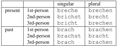
singular plural present 1st-person breche brechen
2nd-person brichst brecht
3rd-person bricht brechen
past 1st-person brach brachen
2nd-person brachst bracht
[image:2.612.82.289.62.142.2]3rd-person brach brachen Table 1: Part of a morphological paradigm in German, showing the spellings of some inflections of the lexeme
b&r ak(whose lemma isbrechen), organized in a grid. Types: In carrying out the above, we will
recon-struct specificmorphological paradigmsof the
lan-guage. A paradigm is a grid of all the inflected forms of some lexeme, as illustrated in Table 1. Our recon-structed paradigms will include our predictions of inflected forms that were never observed in the cor-pus. This tabular information about the types (rather than the tokens) of the language may be separately useful, for example in translation and other genera-tion tasks, and we will evaluate its accuracy.
Grammar: We estimate parameters ~θ that de-scribe general patterns in the language. We learn a prior distribution over inflectional paradigms by learning (e.g.) how a verb’s suffix or stem vowel tends to change when it is pluralized. We also learn (e.g.) whether singular or plural forms are more com-mon. Our basic strategy is Monte Carlo EM, so these parameters tell us how to guess the paradigms (Monte Carlo E step), then these reconstructed paradigms tell us how to reestimate the parameters (M step), and so on iteratively. We use a few supervised paradigms to initialize the parameters and help reestimate them.
2 Overview of the Model
We begin by sketching the main ideas of our model, first reviewing components that we introduced in earlier papers. Sections 5–7 will give more formal details. Full details and more discussion can be found in the first author’s dissertation (Dreyer, 2011).
2.1 Modeling Morphological Alternations
We begin with a family of joint distributionsp(x, y)
over string pairs, parameterized byθ~. For example,
to model just the semi-systematic relation between a
German lemma and its3rd-person singular present
form, one could train~θto maximize the likelihood
of(x, y)pairs such as (brechen,bricht). Then,
given a lemmax, one could predict its inflected form
yviap(y|x), and vice-versa.
Dreyer et al. (2008) define such a family via a log-linear model with latent alignments,
p(x, y) =X
a
p(x, y, a)∝X
a
exp(~θ·f~(x, y, a))
Herearanges over monotonic 1-to-1 character
align-ments betweenxandy.∝means “proportional to” (p
is normalized to sum to 1).f~extracts a vector of local
features from the aligned pair by examining trigram
windows. Thus ~θ can reward or penalize specific
features—e.g., insertions, deletions, or substitutions
in specific contexts, as well as trigram features ofx
andyseparately.3 Inference and training are done by
dynamic programming on finite-state transducers. 2.2 Modeling Morphological Paradigms
A paradigm such as Table 1 describes how some
ab-stract lexeme (b&r ak) isexpressedin German.4 We
evaluatewhole paradigmsas linguistic objects,
fol-lowing word-and-paradigm or realizational morphol-ogy (Matthews, 1972; Stump, 2001). That is, we
pre-sume that some language-specific distributionp(π)
defines whether a paradigmπis a grammatical—and
a priorilikely—way for a lexeme to express itself
in the language. Learningp(π)helps us reconstruct
paradigms, as described at the end of section 1.2. Letπ= (x1, x2, . . .). In Dreyer and Eisner (2009),
we showed how to model p(π) as a renormalized
productof many pairwise distributionsprs(xr, xs), each having the log-linear form of section 2.1:
p(π)∝Y
r,s
prs(xr, xs)∝exp(
X
r,s
~
θ·−→frs(xr, xs, ars))
This is an undirected graphical model (MRF) over string-valuedrandom variablesxs; each factorprs evaluates the relationship between some pair of strings. Note that it is still a log-linear model, and
pa-rameters in~θcan be reused across differentrspairs.
To guess at unknown strings in the paradigm, Dreyer and Eisner (2009) show how to perform ap-proximate inference on such an MRF by loopy belief
3Dreyer et al. (2008) devise additional helpful features based on enriching the aligned pair with additional latent information, but our present experiments drop those for speed.
X1pl
X2pl
X3pl
XLem
X1sg
X2sg
X3sg
brichen brechen
...
?
brichen brechen
...
?
bricht brecht
...
?
briche breche
...
?
brichst brechst
...
?
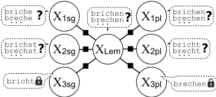
[image:3.612.77.290.63.159.2]bricht brechen
Figure 1: A distribution over paradigms modeled as an MRF over 7 strings. Random variables XLem, X1st, etc.,
are thelemma, the1st personform, etc. Suppose two forms are observed (denoted by the “lock” icon). Given these observations, belief propagation estimates the poste-rior marginals over the other variables (denoted by “?”).
propagation, using finite-state operations. It is not
necessary to include allrspairs. For example, Fig. 1
illustrates the result of belief propagation on a simple MRF whose factors relate all inflected forms to a common (possibly unobserved) lemma, but not
di-rectly to one another.5
Our method could be used with anyp(π). To speed
up inference (see footnote 7), our present experiments
actually use thedirectedgraphical model variant of
Fig. 1—that is,p(π) =p1(x1)·Qs>1p1s(xs |x1),
wherex1denotes the lemma.
2.3 Modeling the Lexicon (types)
Dreyer and Eisner (2009) learnedθ~by partially
ob-serving some paradigms (type data). That work, while rather accurate at predicting inflected forms, sometimes erred: it predicted spellings that never oc-curred in text, even for forms that “should” be com-mon. To fix this, we shall incorporate an unlabeled or POS-tagged corpus (token data) into learning.
We therefore need a model for generating tokens— aprobabilistic lexiconthat specifies which inflections of which lexemes are common, and how they are spelled. We do not know our language’s probabilistic lexicon, but we assume it was generated as follows:
1. Choose parameters~θof the MRF. This defines
p(π): which paradigms are likelya priori.
2. Choose a distribution over the abstract lexemes.
5This view is adopted by some morphological theorists (Al-bright, 2002; Chan, 2006), although see Appendix E.2 for a caution about syncretism. Note that when the lemma is unob-served, the other forms do still influence one another indirectly.
3. For each lexeme, choose a distribution over its inflections.
4. For each lexeme, choose a paradigm that will be used to express the lexeme orthographically.
Details are given later. Briefly, step 1 samples~θ
from a Gaussian prior. Step 2 samples a distribution from a Dirichlet process. This chooses a countable number of lexemes to have positive probability in the language, and decides which ones are most common. Step 3 samples a distribution from a Dirichlet. For
the lexeme think, this might choose to make
1st-person singularmore common than for typical verbs.
Step 4 just samples IID fromp(π).
In our model, each part of speech generates its own
lexicon: VERBs are inflected differently fromNOUNs
(different parameters and number of inflections). The
size and layout of (e.g.)VERBparadigms is
language-specific; we currently assume it is given by a linguist,
along with a few supervisedVERBparadigms.
2.4 Modeling the Corpus (tokens)
At present, we use only a very simple exchangeable model of the corpus. We assume that each word was independently sampled from the lexicon given its part of speech, with no other attention to context.
For example, a token ofbrechenmay have been
chosen by choosing frequent lexemeb&r akfrom the
VERBlexicon; then choosing1st-person pluralgiven
b&r ak; and finally looking up that inflection’s spelling inb&r ak’s paradigm. This final lookup is determinis-tic since the lexicon has already been generated.
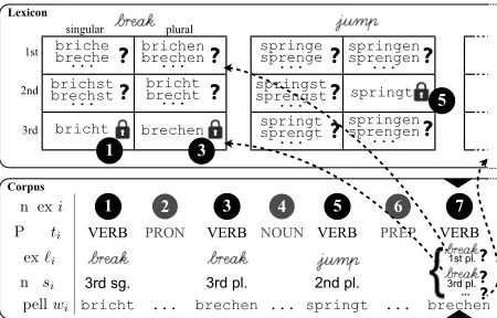
3 A Sketch of Inference and Learning 3.1 Gibbs Sampling Over the Corpus
singular plural
1st
2nd
3rd bricht brichst brechst... ?
briche breche... ?
brechen bricht brecht... ? brichen brechen... ?
springst sprengst... ?
springe sprenge... ?
springt sprengt... ?
springen sprengen...
springen sprengen...
1 3
Indexi 2
PRON
4 NOUN
6 PREP
POSti
Inflsi
Spellwi
[image:4.612.73.298.64.208.2]Lex�i 1 VERB 3rd sg. bricht 5 VERB 2nd pl. springt 3 VERB 3rd pl. brechen ? ? 5 Lexicon Corpus ? ... ? ? springt 7 VERB 1st pl. ... brechen ... ... ... 3rd pl.
Figure 2: A state of the Gibbs sampler (note that the assumed generative process runs roughly top-to-bottom). Each corpus tokenihas been tagged with part of speechti,
lexeme`iand inflectionsi. Token¶has been tagged as
b&r akand3rd sg., which locked the corresponding type spelling in the paradigm to the spellingw1 =bricht;
similarly for¸andº. Noww7is about to be reanalyzed.
The key intuition is that the current analyses of the otherverb tokens imply a posterior distribution over
theVERBlexicon, shown in the top half of the figure.
First, because of the current analyses of¶and¸,
the 3rd-personspellings of b&r ak are already
con-strained to matchw1 andw3(the “lock” icon).
Second, belief propagation as in Fig. 1 tells us
which other inflections of b&r ak(the “?” icon) are
plausibly spelled asbrechen, and how likely they
are to be spelled that way.
Finally, the fact that other tokens are associated withb&r aksuggest that this is a popular lexeme,
mak-ing it a plausible explanation of¼as well. (This is
the “rich get richer” property of the Chinese restau-rant process; see section 6.6.) Furthermore, certain
inflections ofb&r akappear to be especially popular.
In short, given the other analyses, we know which
inflected lexemes in the lexicon are likely,andhow
likely each one is to be spelled asbrechen. This lets
us compute the relative probabilities of the possible
analyses of token¼, so that the Gibbs sampler can
accordingly choose one of these analyses at random.
3.2 Monte Carlo EM Training of~θ
For a given~θ, this Gibbs sampler converges to the
posterior distribution over analyses of the full corpus.
To improve our~θestimate, we periodically adjust~θ
to maximize or increase the probability of the most
recent sample(s). For example, having taggedw5=
springtass5 =2nd-person pluralmay strengthen
our estimated probability that2nd-personspellings
tend to end in-t. That revision to~θ, in turn, will
influence future moves of the sampler.
If the sampler is run long enough between calls to
the~θoptimizer, this is a Monte Carlo EM procedure
(see end of section 1.2). It uses the data to optimize a
language-specific priorp(π)over paradigms—an
em-pirical Bayes approach. (A fully Bayesian approach
would resample~θas part of the Gibbs sampler.)
3.3 Collapsed Representation of the Lexicon
The lexicon iscollapsed outof our sampler, in the
sense that we do not represent a single guess about the infinitely many lexeme probabilities and paradigms. What we store about the lexicon is information about its full posterior distribution: the top half of Fig. 2.
Fig. 2 names its lexemes asb&r akandjumpfor
ex-pository purposes, but of course the sampler cannot reconstruct such labels. Formally, these labels are col-lapsed out, and we represent lexemes as anonymous
objects. Tokens¶and¸are tagged with thesame
anonymous lexeme (which will correspond to sitting at the same table in a Chinese restaurant process).
For each lexeme`and inflections, we maintain
pointers to any tokens currently tagged with the slot (`, s). We also maintain an approximate marginal
distribution over the spelling of that slot:6
1. If(`, s)points to at least one tokeni, then we
know(`, s)is spelled aswi(with probability 1).
2. Otherwise, the spelling of(`, s) is not known.
But if some spellings in`’s paradigm are known,
store a truncated distribution that enumerates the
25 most likely spellings for(`, s), according to
loopy belief propagation within the paradigm.
3. Otherwise, we have observed nothing about`:
it is currently unused. All such`share the same
marginal distribution over spellings of (`, s):
the marginal of the priorp(π). Here a 25-best
list could not cover all plausible spellings. In-stead we store a probabilistic finite-state
lan-guage model that approximates this marginal.7
6Cases 1 and 2 below must in general beupdatedwhenever a slot switches between having 0 and more than 0 tokens. Cases 2 and 3 must be updated when the parameters~θchange.
de-A hash table based on cases 1 and 2 can now be
used to rapidly map any wordwto a list of slots of
existing lexemes that might plausibly have generated
w. To ask whetherwmight instead be an inflections
of a novel lexeme, we scorewusing the probabilistic
finite-state automata from case 3, one for eachs.
The Gibbs sampler randomly chooses one of these analyses. If it chooses the “novel lexeme” option, we create an arbitrary new lexeme object in mem-ory. The number of explicitly represented lexemes is always finite (at most the number of corpus tokens). 4 Interpretation as a Mixture Model
It is common to cluster points inRn by assuming
that they were generated from amixture of Gaussians,
and trying to reconstruct which points were generated from the same Gaussian.
We are similarly clustering word tokens by
assum-ing that they are generated from amixture of weighted
paradigms. After all, each word token was obtained by randomly sampling a weighted paradigm (i.e., a cluster) and then randomly sampling a word from it. Just as each Gaussian in a Gaussian mixture is
a distribution over all points Rn, each weighted
paradigm is a distribution over all spellingsΣ∗(but
assigns probability>0to only a finite subset ofΣ∗).
Inference under our model clusters words together by tagging them with the same lexeme. It tends to group words that are “similar” in the sense that the
base distributionp(π)predicts that they would tend
to co-occur within a paradigm. Suppose a corpus contains several unlikely but similar tokens, such as discombobulated and discombobulating. A language might have one probable lexeme from whose paradigm all these words were sampled. It is much less likely to have several probable lexemes that allcoincidentallychose spellings that started with discombobulat-. Generating discombobulat-only once is cheaper (especially for such a long pre-fix), so the former explanation has higher probability.
This is like explaining nearby points inRnas
sam-ples from the same Gaussian. Of course, our model is sensitive to more than shared prefixes, and it does not merely cluster words into a paradigm but assigns them to particular inflectional slots in the paradigm.
fined as at the end of section 2.2. If not, one could still try belief propagation; or one could approximate by estimating a language model from the spellings associated with slotsby cases 1 and 2.
4.1 The Dirichlet Process Mixture Model
Our mixture model uses aninfinitenumber of
mix-ture components. This avoids placing a prior bound on the number of lexemes or paradigms in the lan-guage. We assume that a natural language has an infinite lexicon, although most lexemes have suffi-ciently low probability that they have not been used in our training corpus or even in human history (yet).
Our specific approach corresponds to a Bayesian technique, the Dirichlet process mixture model. Ap-pendix A (supplementary material) explains the DPMM and discusses it in our context.
The DPMM would standardly be presented as gen-erating a distribution over countably many Gaussians or paradigms. Our variant in section 2.3 instead broke this into two steps: it first generated a distribution over countably many lexemes (step 2), and then gen-erated a weighted paradigm for each lexeme (steps 3–4). This construction keeps distinct lexemes sepa-rate even if they happen to have identical paradigms (polysemy). See Appendix A for a full discussion.
5 Formal Notation 5.1 Value Types
We now describe our probability model in more for-mal detail. It considers the following types of mathe-matical objects. (We use consistent lowercase letters for values of these types, and consistent fonts for constants of these types.)
Aword w, such asbroken, is a finite string of
any length, over some finite, given alphabetΣ.
Apart-of-speech tagt, such asVERB, is an
ele-ment of a certain finite setT, which in this paper we
assume to be given.
Aninflections,8such aspast participle, is an
ele-ment of a finite setSt. A token’s part-of-speech tag
t ∈ T determines its setSt of possible inflections.
For tags that do not inflect,|St| = 1. The sets St
are language-specific, and we assume in this paper that they are given by a linguist rather than learned. A linguist also specifies features of the inflections: the grid layout in Table 1 shows that 4 of the 12
inflections inSVERB share the “2nd-person” feature.
Aparadigmfort∈ T is a mappingπ:St→Σ∗,
specifying aspellingfor each inflection inSt. Table 1
shows oneVERBparadigm.
Alexeme`is an abstract element of some lexical
spaceL. Lexemes have no internal semantic
struc-ture: the only question we can ask about a lexeme is whether it is equal to some other lexeme. There is no upper bound on how many lexemes can be discovered
in a text corpus;Lis infinite.
5.2 Random Quantities
Our generative model of the corpus is a joint probabil-ity distribution over a collection of random variables. We describe them in the same order as section 1.2.
Tokens:The corpus is represented bytoken
vari-ables. In our setting the sequence of wordsw~ =
w1, . . . , wn ∈ Σ∗ is observed, along with n. We must recover the corresponding part-of-speech tags ~t = t1, . . . , tn ∈ T, lexemes~` = `1, . . . , `n ∈ L,
and inflections~s=s1, . . . , sn, where(∀i)si ∈ Sti.
Types: The lexicon is represented by type variables. For each of the infinitely many
lex-emes ` ∈ L, and each t ∈ T, the paradigm
πt,` is a function St → Σ∗. For example,
Table 1 shows a possible value πVERB,b&r ak.
The various spellings in the paradigm, such as πVERB,b&r ak(1st-person sing. pres.)=breche, are string-valued random variables that are correlated with one another.
Since the lexicon is to be probabilistic (section 2.3),
Gt(`)denotes tagt’s distribution over lexemes`∈
L, whileHt,`(s)denotes the tagged lexeme(t, `)’s
distribution over inflectionss∈ St.
Grammar: Global properties of the language are
captured bygrammarvariables that cut across
lex-ical entries: our parameters~θthat describe typical
inflectional alternations, plus parametersφ~t, αt, α0
t, ~τ (explained below). Their values control the overall shape of the probabilistic lexicon that is generated.
6 The Formal Generative Model
We now fully describe the generative process that was sketched in section 2. Step by step, it randomly chooses an assignment to all the random variables of section 5.2. Thus, a given assignment’s probability— which section 3’s algorithms consult in order to re-sample or improve the current assignment—is the
product of the probabilities of the individual choices, as described in the sections below. (Appendix B provides a drawing of this as a graphical model.)
6.1 Grammar Variablesp(~θ), p(−→φt), p(αt), p(α0t) First select the grammar variables from a prior. (We will see below how these variables get used.) Our
experiments used fairly flat priors. Each weight in~θ
or−→φtis drawn IID fromN(0,10), and eachαtorα0t
from a Gamma with mode 10 and variance 1000.
6.2 Paradigmsp(πt,` |~θ)
For eacht ∈ T, let Dt(π) denote the distribution
over paradigms that was presented in section 2.2
(where it was calledp(π)). Dtis fully specified by
our graphical model for paradigms of part of speech
t, together with its parameters~θas generated above.
This is the linguistic core of our model. It
consid-ers spellings:DVERBdescribes what verb paradigms
typically look like in the language (e.g., Table 1).
Parameters in ~θ may be shared across parts of
speecht. These “backoff” parameters capture
gen-eral phonotactics of the language, such as prohibited letter bigrams or plausible vowel changes.
For each possible tagged lexeme (t, `), we now
draw a paradigmπt,`fromDt. Most of these lexemes
will end up having probability 0 in the language.
6.3 Lexical Distributionsp(Gt|αt)
We now formalize section 2.3. For eacht∈ T, the
language has a distributionGt(`)over lexemes. We
drawGtfrom a Dirichlet process DP(G, αt), where
Gis the base distribution over L, and αt > 0 is
aconcentration parametergenerated above. Ifαt
is small, thenGtwill tend to have the property that
most of its probability mass falls on relatively few
of the lexemes inLt =def {` ∈ L : Gt(`) > 0}. A
closed-class tagis one whoseαtis especially small.
ForGto be a uniform distribution over an infinite
lexeme setL, we needLto be uncountable.9
How-ever, it turns out10 that with probability 1, eachL
t iscountablyinfinite, and all theLtare disjoint. So
each lexeme`∈ Lis selected by at most one tagt.
9For example,
Ldef= [0,1], so thatb&r akis merely a sugges-tive nickname for a lexeme such as 0.2538159.
6.4 Inflectional Distributionsp(Ht,`|−→φt, α0t)
For each tagged lexeme(t, `), the language specifies
some distributionHt,` over its inflections.
First we construct backoff distributionsHtthat are
independent of`. For each tagt∈ T, letHtbe some
base distribution over St. AsSt could be large in
some languages, we exploit its grid structure (Table 1)
to reduce the number of parameters ofHt. We take
Htto be a log-linear distribution with parameters−→φt
that refer to featuresof inflections. E.g., the
2nd-personinflections might besystematicallyrare.
Now we model eachHt,`as an independent draw
from a finite-dimensional Dirichlet distribution with
meanHtand concentration parameterα0t. E.g.,think
might be biased toward1st-person sing. present.
6.5 Part-of-Speech Tag Sequencep(~t|~τ)
In our current experiments,~tis given. But in general,
to discover tags and inflections simultaneously, we
can suppose that the tag sequence~t(and its lengthn)
are generated by a Markov model, with tag bigram or
trigram probabilities specified by some parameters~τ.
6.6 Lexemesp(`i |Gti)
We turn to section 2.4. A lexeme token depends on its tag: draw`i fromGti, sop(`i|Gti) =Gti(`i).
6.7 Inflectionsp(si|Hti,`i)
An inflection slot depends on its tagged lexeme: we drawsifromHti,`i, sop(si |Hti,`i) =Hti,`i(si).
6.8 Spell-outp(wi|πti,`i(si))
Finally, we generate the wordwithrough a
determin-isticspell-outstep.11 Given the tag, lexeme, and
in-flection at positioni, we generate the wordwisimply
by looking up its spelling in the appropriate paradigm. Sop(wi|πti,`i(si))is 1 ifwi =πti,`i(si), else 0.
6.9 Collapsing the Assignment
Again, afullassignment’s probability is the product
of all the above factors (see drawing in Appendix B).
11To account for typographical errors in the corpus, the spell-out process could easily be made nondeterministic, with the observed wordwiderived from the correct spellingπti,`i(si)
by a noisy channel model (e.g., (Toutanova and Moore, 2002)) represented as a WFST. This would make it possible to analyze
brkoenas a misspelling of a common or contextually likely word, rather than treating it as an unpronounceable, irregularly inflected neologism, which is presumably less likely.
But computationally, our sampler’s state leaves the Gtunspecified. So its probability is the integral of
p(assignment)over all possibleGt. AsGtappears only in the factors from headings 6.3 and 6.6, we can
just integrate it out oftheirproduct, to get a collapsed
sub-model that generatesp(~`|~t, ~α)directly:
Z
GADJ
· · · Z
GVERB
dG Y
t∈T
p(Gt|αt)
! n
Y
i=1
p(`i |Gti)
!
=p(~`|~t, ~α) =
n
Y
i=1
p(`i|`1, . . . `i−1~t, ~α)
where it turns out that the factor that generates`iis
proportional to|{j < i:`j =`iandtj =ti}|if that
integer is positive, else proportional toαtiG(`i).
Metaphorically, each tagtis aChinese restaurant
whosetablesare labeled with lexemes. The tokens
are hungrycustomers. Each customeri= 1,2, . . . , n
enters restaurantti in turn, and`idenotes the label
of the table she joins. She picks an occupied table with probability proportional to the number of pre-vious customers already there, or with probability
proportional toαtishe starts a new table whose label
is drawn fromG(it is novel with probability 1, since
Ggives infinitesimal probability to each old label).
Similarly, we integrate out the infinitely many
lexeme-specific distributionsHt,`from the product of
6.4 and 6.7, replacing it by the collapsed distribution p(~s|~`,~t,−→φt,−→α0) [recall that−→φ
tdeterminesHt]
=
n
Y
i=1
p(si |s1, . . . si−1, ~`, ~t,φ−→t,−→α0)
where the factor forsi is proportional to|{j < i :
sj =siand(tj, `j) = (ti, `i)}|+α0tiHti(si).
Metaphorically, each table`in Chinese restaurant
thas a fixed, finite set ofseatscorresponding to the
inflectionss ∈ St. Each seat is really a bench that
can hold any number of customers (tokens). When
customerichooses to sit at table`i, she also chooses
a seatsi at that table (see Fig. 2), choosing either an
already occupied seat with probability proportional to the number of customers already in that seat, or else
a random seat (sampled fromHtiand not necessarily
empty) with probability proportional toα0ti.
7 Inference and Learning
sample from the posterior of(~s, ~`, ~t)givenw~ and the grammar variables, and an M step that adjusts the grammar variables to maximize the probability of the (w, ~s, ~`, ~t)~ samples given those variables.
7.1 Block Gibbs Sampling
As in Gibbs sampling for the DPMM, our sampler’s
basic move is to reanalyze token i(see section 3).
This corresponds to making customeriinvisible and
then guessing where she is probably sitting—which
restaurantt, table`, and seats?—given knowledge
ofwiand the locations of all other customers.12
Concretely, the sampler guesses location(ti, `i, si)
with probabilityproportionalto the product of
• p(ti |ti−1, ti+1, ~τ)(from section 6.5)
• the probability (from section 6.9) that a new
cus-tomer in restauranttichooses table`i, given the
othercustomers in that restaurant (andαti)13
• the probability (from section 6.9) that a new
customer at table`i chooses seatsi, given the
othercustomers at that table (and−→φtiandα0ti)
13
• the probability (from section 3.3’s belief
propa-gation) thatπti,`i(si) =wi(given~θ).
We sample only from the(ti, `i, si)candidates for
which the last factor is non-negligible. These are found with the hash tables and FSAs of section 3.3. 7.2 Semi-Supervised Sampling
Our experiments also consider the semi-supervised
case where a fewseed paradigms—typedata—are
fully or partially observed. Our samples should also be conditioned on these observations. We assume that our supervised list of observed paradigms was
generated by sampling fromGt.14 We can modify
our setup for this case: certain tables have ahost
who dictates the spelling of some seats and attracts appropriate customers to the table. See Appendix C. 7.3 Parameter Gradients
Appendix D gives formulas for the M step gradients.
12Actually, to improve mixing time, we choose a currently active lexeme`uniformly at random, makeallcustomers{i:
`i=`}invisible, and sequentially guess where they are sitting.
13This is simple to find thanks to the exchangeability of the CRP, which lets us pretend thatientered the restaurant last.
14Implying that they are assigned to lexemes with non-negligible probability. We would learn nothing from a list of merelypossibleparadigms, sinceLtis infinite and every
con-ceivable paradigm is assigned tosome`∈ Lt(in fact many!).
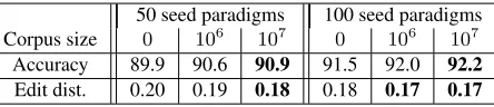
50 seed paradigms 100 seed paradigms Corpus size 0 106 107 0 106 107
Accuracy 89.9 90.6 90.9 91.5 92.0 92.2
[image:8.612.318.540.62.110.2]Edit dist. 0.20 0.19 0.18 0.18 0.17 0.17
Table 2: Whole-word accuracy and edit distance of pre-dicted inflection forms given the lemma. Edit distance to the correct form is measured in characters. Best numbers per set of seed paradigms in bold (statistically signifi-cant on our large test set under a paired permutation test,
p < 0.05). Appendix E breaks down these results per
inflection and gives an error analysis and other statistics. 8 Experiments
8.1 Experimental Design
We evaluated how well our model learns German
verbal morphology. As corpus we used the first 1
million or 10 million words from WaCky (Baroni
et al., 2009). Forseed and test paradigmswe used
verbal inflectional paradigms from the CELEX mor-phological database (Baayen et al., 1995). We fully observed the seed paradigms. For each test paradigm,
we observed thelemmatype (Appendix C) and
eval-uated how well the system completed the other 21 forms (see Appendix E.2) in the paradigm.
We simplified inference by fixing the POS tag sequence to the automatic tags delivered with the WaCky corpus. The result that we evaluated for each variable was the value whose probability, averaged
over the entire Monte Carlo EM run,15was highest.
For more details, see (Dreyer, 2011).
All results are averaged over 10 different train-ing/test splits of the CELEX data. Each split sampled 100 paradigms as seed data and used the
remain-ing 5,415 paradigms for evaluation.16 From the 100
paradigms, we also sampled 50 to obtain results with
smaller seed data.17
8.2 Results
Type-based Evaluation. Table 2 shows the results of predicting verb inflections, when running with no
corpus, versus with an unannotated corpus of size106
and107 words. Just using 50 seed paradigms, but
15This includes samples from before~θhas converged, some-what like the voted perceptron (Freund and Schapire, 1999).
Bin Frequency # Verb Forms
1 0–9 116,776
2 10–99 4,623
3 100–999 1,048
4 1,000–9,999 95
5 10,000– 10
[image:9.612.109.261.62.143.2]all any 122,552
Table 3: The inflected verb forms from 5,615 inflectional paradigms, split into 5 token frequency bins. The frequen-cies are based on the 10-million word corpus.
no corpus, gives an accuracy of 89.9%. By adding a corpus of 10 million words we reduce the error rate by 10%, corresponding to a one-point increase in absolute accuracy to 90.9%. A similar trend can be seen when we use more seed paradigms. Sim-ply training on 100 seed paradigms, but not using a corpus, results in an accuracy of 91.5%. Adding a corpus of 10 million words to these 100 paradigms re-duces the error rate by 8.3%, increasing the absolute accuracy to 92.2%. Compared to the large corpus, the smaller corpus of 1 million words goes more than half the way; it results in error reductions of 6.9% (50 seed paradigms) and 5.8% (100 seed paradigms). Larger unsupervised corpora should help by increas-ing coverage even more, although Zipf’s law implies
a diminishing rate of return.18
We also tested a baseline that simply inflects each morphological form according to the basic regular German inflection pattern; this reaches an accuracy of only 84.5%.
Token-based Evaluation. We now split our results into different bins: how well do we predict the spellings of frequently expressed (lexeme, inflection) pairs as opposed to rare ones? For example, the third
person singular indicative ofgiv(geben) is used
significantly more often than the second person plural
subjunctive ofb$ask(aalen);19they are in different
frequency bins (Table 3). The more frequent a form is in text, the more likely it is to be irregular (Jurafsky et al., 2000, p. 49).
The results in Table 4 show: Adding a corpus of either 1 or 10 million words increases our prediction
accuracy acrossall frequency bins, often
dramati-cally. All methods do best on the huge number of
18Considering the 63,778 distinct spellings from all of our 5,615 CELEX paradigms, we find that the smaller corpus con-tains 7,376 spellings and the10×larger corpus contains 13,572.
19See Appendix F for how this was estimated from text.
50 seed paradigms 100 seed paradigms
Bin 0 106 107 0 106 107 1 90.5 91.0 91.3 92.1 92.4 92.6
2 78.1 84.5 84.4 80.2 85.5 85.1 3 71.6 79.3 78.1 73.3 80.2 79.1 4 57.4 61.4 61.8 57.4 62.0 59.9 5 20.7 25.0 25.0 20.7 25.0 25.0 all 52.6 57.5 57.8 53.4 58.5 57.8
all (e.d.) 1.18 1.07 1.03 1.16 1.02 1.01
Table 4: Token-based analysis: Whole-word accuracy re-sults split into different frequency bins. In the last two rows, all predictions are included, weighted by the fre-quency of the form to predict. Last row is edit distance.
rare forms (Bin 1), which are mostly regular, and worst on on the 10 most frequent forms of the lan-guage (Bin 5). However, adding a corpus helps most in fixing the errors in bins with more frequent and hence more irregular verbs: in Bins 2–5 we observe improvements of up to almost 8% absolute percent-age points. In Bin 1, the no-corpus baseline is already relatively strong.
Surprisingly, while we always observe gains from using a corpus, the gains from the 10-million-word corpus are sometimes smaller than the gains from the 1-million-word corpus, except in edit distance. Why? The larger corpus mostly adds new infrequent types,
biasing~θtoward regular morphology at the expense
of irregular types. A solution might be to model irreg-ular classes with separate parameters, using the latent conjugation-class model of Dreyer et al. (2008).
Note that, by using a corpus, we even improve our prediction accuracy for forms and spellings that
arenotfound in the corpus, i.e.,novelwords. This
is thanks to improved grammar parameters. In the token-based analysis above we have already seen that prediction accuracy increases for rare forms (Bin 1). We add two more analyses that more explicitly show our performance on novel words. (a) We find all paradigms that consist of novel spellings only, i.e. none of the correct spellings can be found in the
corpus.20The whole-word prediction accuracies for
the models that use corpus size 0, 1 million, and 10 million words are, respectively, 94.0%, 94.2%, 94.4% using 50 seed paradigms, and 95.1%, 95.3%, 95.2% using 100 seed paradigms. (b) Another,
[image:9.612.317.537.62.164.2]pler measure is the prediction accuracy on all forms whose correct spelling cannot be found in the 10-million-word corpus. Here we measure accuracies of 91.6%, 91.8% and 91.8%, respectively, using 50 seed paradigms. With 100 seed paradigms, we have 93.0%, 93.4% and 93.1%. The accuracies for the models that use a corpus are higher, but do not al-ways steadily increase as we increase the corpus size. The token-based analysis we have conducted here shows the strength of the corpus-based approach pre-sented in this paper. While the integrated graphi-cal models over strings (Dreyer and Eisner, 2009) can learn some basic morphology from the seed paradigms, the added corpus plays an important role in correcting its mistakes, especially for the more fre-quent, irregular verb forms. For examples of specific errors that the models make, see Appendix E.3.
9 Related Work
Our word-and-paradigm model seamlessly handles nonconcatenative and concatenative morphology alike, whereas most previous work in morphological knowledge discovery has modeled concatenative mor-phology only, assuming that the orthographic form of a word can be split neatly into stem and affixes—a simplifying asssumption that is convenient but often not entirely appropriate (Kay, 1987) (how should one
segment Englishstopping,hoping, orknives?).
Inconcatenativework, Harris (1955) finds mor-pheme boundaries and segments words accordingly, an approach that was later refined by Hafer and Weiss (1974), Déjean (1998), and many others. The unsupervised segmentation task is tackled in the annual Morpho Challenge (Kurimo et al., 2010), where ParaMor (Monson et al., 2007) and Morfessor (Creutz and Lagus, 2005) are influential contenders. The Bayesian methods that Goldwater et al. (2006b, et seq.) use to segment between words might also be applied to segment within words, but have no notion of paradigms. Goldsmith (2001) finds what he calls signatures—sets of affixes that are used with a given
set of stems, for example (NULL,-er, -ing,-s).
Chan (2006) learns sets of morphologically related
words; he calls these setsparadigmsbut notes that
they are not substructured entities, in contrast to the paradigms we model in this paper. His models are restricted to concatenative and regular morphology.
Morphology discovery approaches that han-dle nonconcatenative and irregular phenomena are more closely related to our work; they are rarer. Yarowsky and Wicentowski (2000) identify inflection-root pairs in large corpora without supervi-sion. Using similarity as well as distributional clues,
they identify even irregular pairs liketake/took.
Schone and Jurafsky (2001) and Baroni et al. (2002)
extract whole conflation sets, like “abuse,abused,
abuses, abusive, abusively, . . . ,” which may also be irregular. We advance this work by not only extracting pairs or sets of related observed words, but whole structured inflectional paradigms, in which we can also predict forms that have never been ob-served. On the other hand, our present model does not yet use contextual information; we regard this as a future opportunity (see Appendix G). Naradowsky and Goldwater (2009) add simple spelling rules to the Bayesian model of (Goldwater et al., 2006a), en-abling it to handle some systematically nonconcate-native cases. Our finite-state transducers can handle more diverse morphological phenomena.
10 Conclusions and Future Work
We have formulated a principled framework for si-multaneously obtaining morphological annotation, an unbounded morphological lexicon that fills com-plete structured morphological paradigms with ob-served and predicted words, and parameters of a non-concatenative generative morphology model.
We ran our sampler over a large corpus (10 million words), inferring everything jointly and reducing the prediction error for morphological inflections by up to 10%. We observed that adding a corpus increases the absolute prediction accuracy on frequently occur-ring morphological forms by up to almost 8%. Future extensions to the model could leverage token context for further improvements (Appendix G).
References
A. C. Albright. 2002. The Identification of Bases in Morphological Paradigms. Ph.D. thesis, University of California, Los Angeles.
D. Aldous. 1985. Exchangeability and related topics.
École d’été de probabilités de Saint-Flour XIII, pages 1–198.
C. E. Antoniak. 1974. Mixtures of Dirichlet processes with applications to Bayesian nonparametric problems.
Annals of Statistics, 2(6):1152–1174.
R. H Baayen, R. Piepenbrock, and L. Gulikers. 1995. The CELEX lexical database (release 2)[cd-rom]. Philadel-phia, PA: Linguistic Data Consortium, University of Pennsylvania [Distributor].
M. Baroni, J. Matiasek, and H. Trost. 2002. Unsupervised discovery of morphologically related words based on orthographic and semantic similarity. InProc. of the ACL-02 Workshop on Morphological and Phonological Learning, pages 48–57.
M. Baroni, S. Bernardini, A. Ferraresi, and E. Zanchetta. 2009. The WaCky Wide Web: A collection of very large linguistically processed web-crawled corpora.
Language Resources and Evaluation, 43(3):209–226. David Blackwell and James B. MacQueen. 1973.
Fergu-son distributions via Pòlya urn schemes.The Annals of Statistics, 1(2):353–355, March.
David M. Blei and Peter I. Frazier. 2010. Distance-dependent Chinese restaurant processes. InProc. of ICML, pages 87–94.
E. Chan. 2006. Learning probabilistic paradigms for morphology in a latent class model. InProceedings of the Eighth Meeting of the ACL Special Interest Group on Computational Phonology at HLT-NAACL, pages 69–78.
M. Creutz and K. Lagus. 2005. Unsupervised morpheme segmentation and morphology induction from text cor-pora using Morfessor 1.0.Computer and Information Science, Report A, 81.
H. Déjean. 1998. Morphemes as necessary concept for structures discovery from untagged corpora. In
Proc. of the Joint Conferences on New Methods in Language Processing and Computational Natural Lan-guage Learning, pages 295–298.
Markus Dreyer and Jason Eisner. 2009. Graphical models over multiple strings. InProc. of EMNLP, Singapore, August.
Markus Dreyer, Jason Smith, and Jason Eisner. 2008. Latent-variable modeling of string transductions with finite-state methods. In Proc. of EMNLP, Honolulu, Hawaii, October.
Markus Dreyer. 2011.A Non-Parametric Model for the Discovery of Inflectional Paradigms from Plain Text
Using Graphical Models over Strings. Ph.D. thesis, Johns Hopkins University.
T.S. Ferguson. 1973. A Bayesian analysis of some non-parametric problems.The annals of statistics, 1(2):209– 230.
Y. Freund and R. Schapire. 1999. Large margin classifica-tion using the perceptron algorithm.Machine Learning, 37(3):277–296.
J. Goldsmith. 2001. Unsupervised learning of the mor-phology of a natural language.Computational Linguis-tics, 27(2):153–198.
S. Goldwater, T. Griffiths, and M. Johnson. 2006a. In-terpolating between types and tokens by estimating power-law generators. InProc. of NIPS, volume 18, pages 459–466.
S. Goldwater, T. L. Griffiths, and M. Johnson. 2006b. Contextual dependencies in unsupervised word seg-mentation. InProc. of COLING-ACL.
P.J. Green. 1995. Reversible jump Markov chain Monte Carlo computation and Bayesian model determination.
Biometrika, 82(4):711.
M. A Hafer and S. F Weiss. 1974. Word segmentation by letter successor varieties.Information Storage and Retrieval, 10:371–385.
Z. S. Harris. 1955. From phoneme to morpheme. Lan-guage, 31(2):190–222.
G.E. Hinton. 2002. Training products of experts by min-imizing contrastive divergence. Neural Computation, 14(8):1771–1800.
Klara Janecki. 2000.300 Polish Verbs. Barron’s Educa-tional Series.
E. T. Jaynes. 2003. Probability Theory: The Logic of Science. Cambridge Univ Press. Edited by Larry Bret-thorst.
D. Jurafsky, J. H. Martin, A. Kehler, K. Vander Linden, and N. Ward. 2000. Speech and Language Processing: An Introduction to Natural Language Processing, Com-putational Linguistics, and Speech Recognition. MIT Press.
M. Kay. 1987. Nonconcatenative finite-state morphology. InProc. of EACL, pages 2–10.
M. Kurimo, S. Virpioja, V. Turunen, and K. Lagus. 2010. Morpho Challenge competition 2005–2010: Evalua-tions and results. InProc. of ACL SIGMORPHON, pages 87–95.
P. H. Matthews. 1972.Inflectional Morphology: A Theo-retical Study Based on Aspects of Latin Verb Conjuga-tion. Cambridge University Press.
J. Naradowsky and S. Goldwater. 2009. Improving mor-phology induction by learning spelling rules. InProc. of IJCAI, pages 1531–1536.
J. Pitman and M. Yor. 1997. The two-parameter Poisson-Dirichlet distribution derived from a stable subordinator.
Annals of Probability, 25:855–900.
P. Schone and D. Jurafsky. 2001. Knowledge-free induc-tion of inflecinduc-tional morphologies. InProc. of NAACL, volume 183, pages 183–191.
J. Sethuraman. 1994. A constructive definition of Dirich-let priors. Statistica Sinica, 4(2):639–650.
N. A. Smith, D. A. Smith, and R. W. Tromble. 2005. Context-based morphological disambiguation with ran-dom fields. In Proceedings of HLT-EMNLP, pages 475–482, October.
G. T. Stump. 2001. Inflectional Morphology: A Theory of Paradigm Structure. Cambridge University Press. Y.W. Teh, M.I. Jordan, M.J. Beal, and D.M. Blei. 2006.
Hierarchical Dirichlet processes.Journal of the Ameri-can Statistical Association, 101(476):1566–1581. Yee Whye Teh. 2006. A hierarchical Bayesian language
model based on Pitman-Yor processes. In Proc. of ACL.
K. Toutanova and R.C. Moore. 2002. Pronunciation modeling for improved spelling correction. InProc. of ACL, pages 144–151.