Abstract - On a concrete example the authors present the
application of a fuzzy multiple criteria programming method to solve the problem of determining the optimal production program for a given period. The stages of the presentation are: (1) the choice of production program optimization criteria, (2) the setting up of a general fuzzy multiple criteria linear programming model to solve the problem of optimal production program determination, (3) the Zimmermann-s approach to solving the fuzzy multiple criteria linear programming model, and (4) the procedure of solving the concrete problem by applying the Zimmerman's approach and sensitivity analysis of the obtained optimal solutions. At the end the authors provide the research results and suggest topics for further research in this field.
Index term - fuzzy programming, multiple criteria programming, optimization criteria, production program.
I. INTRODUCTION
Determining the optimal production program is one of the most important activities in industrial enterprises. The idea of production program involves a set of different kinds of products manufactured by a company or intended to be manufactured in a particular time period, as well as the structure of the output. An optimal production programme is a very dynamic phenomenon which can be achieved only by continuing effort to put all the resources (financial, material and human) to the best possible use in view of the market requirements. As the entire process of determining the optimal production program in industrial enterprises is complex and dynamic it must be constantly and carefully considered at the company level.
The company production program importantly affects both its quality of operation and its market position.
The optimization of production programs most frequently involves single-criterion programming – linear and nonlinear. In this study, however, we will use a concrete practical example to point to the multicriteria nature of the problem that requires the application of multicriteria programming methods. In addition to that, we will present the production program optimization procedure by use of fuzzy multicriteria linear programming (FMLP) and the FMLP method itself. In the end we will perform the sensitivity analysis of the obtained compromise solution. Manuscript received December 12, 2008.
Tunjo Perić was with the Faculty of Economics Dubrovnik, University of Split, Republic of Croatia. He is now with the Bakery Sunce, 10437 Bestovje, Rakitje, Rakitska cesta 98, Republic of Croatia. Phone: ++385913370620; fax: ++38513370630; e-mail: [email protected].
Zoran Babić is with the Faculty of Economics, University of Split, 21000 Split, Matice hrvatske 31, Republic of Croatia. E-mail: [email protected].
II. CHOOSING THE CRITERIA TO DETERMINE AN OPTIMAL PRODUCTION PROGRAM
The criteria to determine an optimal production program result from the company’s general business goals as well as its specific production goals. Each company has its own set of goals that differs from others in terms of contents and importance.
In the long run the basic goal of company operation is market survival with a secured growth rate. From such a long term goal, strategic goals are derived that refer to the middle term of one to five years. Strategic goals will solve the concrete problems, for example an increase of market share by a certain percentage, expansion of product range, improved level of staff satisfaction, etc. Strategic goals are achieved by realization of short term operational goals. Operational goals or decision goals can be: maximization of output, maximization of capacity utilization, maximization of profits for a particular period, maximization of productivity, economy and profitability of operation in a particular period, maximization of export revenues, etc. Besides operational goals there are also specific goals of particular functions within the company. Thus for example specific goals of production may be quality maximization, minimization of scrap, minimization of pollution, etc. There are also specific goals in other functions such as marketing, finance, development, etc. In more complex organizational structures these goals can be conflicting to some degree, so that the realization of goals in one function does not contribute to the complete realization of goals in other functions and vice versa. Conflicting goals should be taken into account in decision making. One of the most important decisions is determining the optimal production program for a particular period.
The described operational goals result in the criteria that are the direct measure of goal achievement. Production program optimization criteria can be: output expressed in units (piece, ton, etc.), total revenues expressed in monetary units, profit in monetary units, environment pollution expressed in some units of measurement, scrap expressed in units or tons, etc.
In the case of conflicting goals decision making on optimal production program requires application of the appropriate models and methods of multicriteria programming. If it is impossible to measure the contribution of the decision goals to the achievement of the company strategic goals it is imperative to use models and methods of fuzzy multicriteria programming. In such cases the decision maker plays a specific role in the preparation of the model and application of the multicriteria programming method.
Tunjo Perić, Member, IAENG, Zoran Babić, Member, IAENG
III. MULTICRITERIA LINEAR PROGRAMMING MODEL TO SOLVE THE PROBLEM OF DETERMINING THE OPTIMAL
PRODUCTION PROGRAM
When building the MLP model to solve this kind of problem we have to start from the following assumptions:
1. Production program optimization criteria are given. 2. Limited capacities of machinery, raw materials, labour and market are available.
3. The company intends to produce n products. Let us introduce the following signs:
j
f = criteria for production program optimization (j = 1, ... , k),
ij
c = i coefficient of j criteria function (i = 1, ... , n; j = 1, ... , k),
i
x = quantity of i product (i = 1, ... , n),
il
a = the necessary time for l machine to produce the unit of
i product (l = 1, ... , p; i = 1, ... , n),
it
g = standard expenditure of t material used to produce one unit of i product (i = 1, ... , n; t = 1, ... , q),
i
r = standard expenditure of labour to produce one unit of i product (i = 1, ... , n),
l
b = capacity of l machine (l = 1, ... , p),
t
d = quantity of t material (t = 1, ... , q),
r= labour capacity,
i
m = market capacity – maximal possibility of sale (i = 1, ... , n),
i
a = market capacity – minimal quantity needed (i = 1, ... , n).
Now we can formulate the mathematical multicriteria linear programming model:
(max) f =
⎥
⎦
⎤
⎢
⎣
⎡
∑
∑
= =
n
i i ik i
n
i
i
x
c
x
c
1 1
1
,...,
s.t:
l i n
i
il
x
b
a
≤
∑
=1
(l = 1, ... , p)
1
n
it i t i
g x
d
=
≤
∑
(t = 1, ... , q)1
n
i i i
r x
r
=
≤
∑
i i i
a
≤
x
≤
m
(i = 1, ... , n)xi
≥
0 (i = 1, ... , n).The above model will allow us to solve the problem of optimal production program for a particular period by application of multicriteria linear programming (MLP) methods.
IV. CASE STUDY
A. Setting the problem
A textile manufacturing enterprise intends to produce 30 different products (marked 1-30) in the period from January to December.
The net sale price and profit per product are shown in the Table 1.
Table 1. Net sale price and profit per product
The profit indicator per product is calculated on the basis of the planned production program structure, the planned sale prices, and the planned costs. It is assumed that changes in the structure of production program will not significantly affect this indicator.
The production plant of the given enterprise consists of three groups of machines. The first group belongs to the Cutting Unit with 18 cutting machines. The second group belongs to the Sewing Unit with 314 sewing machines. The third group belongs to the Finishing Unit with 48 finishing machines. All the three units work in two shifts. It is anticipated that in the given period the capacity utilization of all the machines will be 80% (taking into account the waste of time occurring in production due to various technical, organizational, market, and other factors).
[image:2.595.305.555.619.783.2]The needed time to manufacture the particular products on the given groups of machines and the capacity of units are shown in the Table 2.
Table 2. Manufacturing time and machine capacity in minutes
Product Cutting Unit
(ai1)
Sewing Unit
(ai2)
Finishing Unit (ai3)
1 0.90 18.40 2.20
2 0.60 19.20 2.21
3 1.80 18.70 2.80
4 0.70 6.70 0.90
5 0.90 7.10 0.50
6 0.30 4.00 0.80
7 0.30 7.20 0.80
8 0.20 5.00 0.50
9 0.20 4.60 0.60
Product (xi)
Net sale price in mon. units
3
( )ci
Profit in mon. units (ci2)
Product (xi)
Net sale price in mon. units
3
( )ci
Profit in mon. units (ci2)
1 3.50 0.60 16 0.75 0.06
2 3.30 0.54 17 0.98 0.12
3 3.60 0.56 18 2.77 0.45
4 1.80 0.25 19 1.37 0.29
5 1.60 0.25 20 1.58 0.31
6 0.80 0.12 21 2.65 0.45
7 0.70 0.08 22 2.20 0.36
8 0.70 0.08 23 1.55 0.20
9 0.80 0.08 24 1.39 0.25
10 0.30 14.40 2.30
11 2.30 11.90 2.00
12 0.60 26.40 2.60
13 0.20 3.10 0.60
14 0.20 3.20 0.50
15 0.10 3.40 1.00
16 0.10 3.30 0.50
17 0.70 5.20 0.70
18 1.00 21.20 1.80
19 0.80 12.90 2.70
20 0.70 12.60 1.40
21 0.80 18.50 2.40
22 0.60 10.10 1.60
23 0.60 17.50 1.80
24 0.30 15.90 1.80
25 1.40 19.50 2.40
26 0.50 15.60 4.20
27 0.20 5.90 3.80
28 0.30 4.40 1.60
29 0.30 4.40 1.60
30 1.90 13.50 2.00
Available machine capacity
3136320 (b1)
54711360 (b2)
8363520 (b3)
In the given period, labour is not a restraining condition for this enterprise.
[image:3.595.46.292.501.790.2]The products from the production program are made of three basic kinds of materials, which can be a restraining condition. The needed quantity of the single kind of material, as well as the maximal quantity that can be purchased by the company (considering the possibility of import and the current contracts with domestic suppliers), are shown in the Table 3.
Table 3. The needed quantity of material per product and the maximal quantity of purchase in kg
Product „A“ (gi1)
„B“ (gi2)
„C“ (gi3)
1 0.016 0.548 - 2 - 0.597 - 3 0.477 0.020 -
4 0.343 - -
5 0.286 - -
6 - 0.134 - 7 - 0.075 - 8 - 0.056 -
9 - 0.012 0.083
10 - 0.647 - 11 - 0.006 0.683
12 - - 0.684
13 0.452 - -
14 - 0.009 0.081 15 - 0.048 - 16 - 0.069 - 17 - 0.037 -
18 1.200 - -
19 0.012 0.362 -
20 0.050 - 0.290
21 0.051 - 0.263
22 - 0.358 -
23 - - 0.291
24 0.012 0.143 -
25 0.012 0.205 -
26 - 0.599 -
27 0.017 0.114 -
28 - 0.114 -
29 0.131 - -
30 0.210 - -
Maximal quantity to be
purchased
538000 (d1)
523000 (d2)
179000 (d3)
The company has limitations in terms of sale possibility, so that in the given period it can at the most sell 500000 pieces of the product 1; 500000 pieces of the product 2; 500000 pieces of the product 3; 345000 pieces of the product 4; 575000 of the product 5; 500000 pieces of the product 6; 500000 pieces of the product 7; 172500 pieces of the product 8; 500000 pieces of the product 9; 500000 of the product 10; 500000 pieces of the product 11; 500000 pieces of the product 12; 500000 pieces of the product 13; 500000 pieces of the product 14; 230000 pieces of the product 15; 500000 pieces of the product 16; 500000 pieces of the product 17; 500000 pieces of the product 18; 500000 pieces of the product 19; 500000 pieces of the product 20; 500000 pieces of the product 21; 500000 pieces of the product 22; 500000 pieces of the product 23; 500000 pieces of the product 24; 500000 pieces of the product 25; 345000 pieces of the product 26; 230000 pieces of the product 27; 300000 pieces of the product 28; 264500 pieces of the product 29 and 500000 pieces of the product 30. According to the current contracts the company has to produce at least 115000 pieces of the product 6; 172500 pieces of the product 13 and 115000 pieces of the product 16.
When making the decision on production program optimization for the given time period the company has determined the following goals: (1) maximization of output, (2) maximization of profit, and (3) maximization of total revenues.
From the production program optimization goals defined in such a way optimization criteria will be derived: (1) output in pieces, (2) profit in monetary units, and (3) total revenues in monetary units.
B. Setting the model to solve the concrete problem According to the stated indicators it is obvious that we have to form a multicriteria linear programming model. Let
i
x = the quantity of i product (i = 1, ... , 30). Then: a) Criteria functions
30 30 30
2 3
1 1 1
(max) i; i i; i i
i i i
f x c x c x
= = =
⎡ ⎤
= ⎢ ⎥
⎣
∑ ∑
∑
⎦,b) Constraints
30
1 1 1
;
i i i
a x b
= ≤
∑
30 2 2 1i i i
a x b
= ≤
∑
; 30 3 31
i i i
a x b
= ≤
∑
;30
1 1
1 i i
i
g x d
= ≤
∑
; 30 2 2 1 i ii
g x d
= ≤
∑
; 30 3 3 1 i ii
d x d
= ≤
∑
; x1≤500000,2 500000,
6 500000,
x ≤ x7 ≤500000, x8 ≤172500, x9≤500000,
10 500000,
x ≤ x11≤500000, x12≤500000, x13≤500000,
14 500000,
x ≤ x15≤230000, x16≤500000, x17≤500000,
18 500000,
x ≤ x19≤500000, x20≤500000, x21≤500000,
22 500000,
x ≤ x23≤500000, x24≤500000, x25≤500000,
26 345000,
x ≤ x27≤230000, x28≤300000, x29≤264500,
30 500000,
x ≤ x6 ≥115000, x13≥172500, x16≥115000,
1,..., 30 0
x x ≥ .
C. Model solving
The presented model is firstly solved by application of the linear programming method maximizing each of the three criteria functions separately on the given set of constraints. The obtained results are:
Table 4. Values of variables and criteria functions Values of criteria functions
Solu-tion Values of variables
1
f f2 f3
1
x x3 =500000,
4 345000,
x =
6 115000,
x =
8 172500,
x =
9 500000,
x =
10 322190,
x =
13 208580,
x =
14 500000,
x =
15 230000,
x =
16 500000,
x =
21 368821,
x =
24 500000,
x =
27 133626,
x =
28 300000,
x =
29 264500,
x =
30 264500
x =
7142644 (100%)
1361995 (79%
* 2
f )
9287307 (90% f3*)
2
x x3 =500000,
5 522309,
x =
6 115000
x =
10 458209,
x =
12 69444,
x =
13 172500,
x =
15 230000,
x =
16 115000,
x =
17 220375,
x =
21 500000,
x =
24 500000,
x =
25 500000,
x =
29 264500
x =
4167337 (58%
* 1
f )
1728671 (100%)
9655347 (94%
* 3
f )
3
x x3 =500000,
4 345000,
x =
6 115000,
x =
5551435 (78%
* 1
f )
1637435 (95%
* 2)
f
10260245 (100%)
8 172500,
x =
9 500000,
x =
10 322190,
x =
13 208580,
x =
14 500000,
x =
15 230000,
x =
16 500000,
x =
21 368821,
x =
24 500000,
x =
25 500000,
x =
27 133626,
x =
28 300000,
x =
29 264500,
x =
30 91218
x =
From the table 4 it is obvious that by maximizing the function f1 we obtain the value for that function which is significantly different from the value of that function when we maximize the functions f2 and f3, respectively. The
significant difference in values of the single criteria functions exists even when the other two criteria functions are maximized. This reveals the conflict of the set goals and the need to apply a multicriteria programming method when solving this concrete model. Namely, the company which has to adopt one solution without using multicriteria programming has a choice that is limited only to marginal solutions, which, as we can see in this example, differ significantly. On the other hand, solving the model by use of multicriteria programming methods we will obtain solutions that from the decision maker's viewpoint provide more acceptable values of criteria functions. We will here present the procedure of determining optimal production program by application of Zimmerman's approach to solving fuzzy multicriteria programming model.
Solving the model by Zimmerman's fuzzy multi-criteria programming approach
We will first present the theoretical foundation of this approach to solving MLP models. Then we will show how to use this approach in solving the production program optimization model for the textile manufacturing company and perform sensitivity analysis of the obtained compromise solution.
Zimmerman [13] was the first to use the maximin operator of Bellman and Zadeh [2] to solve multicriteria models. The MLP model can be presented in the following form (Lai and Hwang [6]):
[
1 2]
max/ min f x( ), f x( ) , ,… fK( )x
s.t. (1)
{
}
{
s( ) , , 0, 1, ,}
, x∈X = ⎪x g x ≥ = ≤ s= … mwhere f xj( ), j ∈ J, are criteria functions which have to be maximised,f xi( ), i∈I, are criteria functions that have to be minimised, and IUJ=
{
1, ,… K}
. Functions f xk( )and( ),
s
g x (k = 1, ... ,K; s = 1, ... ,m) can be linear or non-linear. Zimmerman considered the model (1) as:
so that ( ) 0,
k k
f x f k
≈
> ∀ (2)
, x∈X where 0,
k
f ∀k are the appropriate goals. It is assumed that all the criteria functions are maximised. Here the criteria functions in the equation (1) are considered as fuzzy constraints. If the tolerances of fuzzy constraints are given, their membership functions μk( )x can be founded for ∀k. Considering the concept of min-operator, the set of allowable solutions is defined by intersection of the fuzzy goal set. This set of allowable solutions is thus defined by its
membership functionμD( ),x which is
1
( ) min( ( ), , ( )).
D x x K x
μ = μ … μ Consequently, the decision
maker makes the decision with the minimal μD value in the
set of allowable solutions. The chosen solution can be obtained by solving the model maximising μD( )x on the set of allowable solutions. That is:
max min k( )
k μ x
⎡ ⎤
⎣ ⎦, s.t. x∈X. (3) Let min k( )
k x
α = μ be the generally satisfactory level of compromise. Then (3) results in:
maxα s.t.
( ),
k x k
α μ≤ ∀ (4) .
x∈X
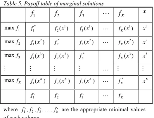
[image:5.595.41.305.425.627.2]To found the membership functions of criteria functions we will firstly form the payoff table of marginal solutions, as shown in the following table:
Table 5. Payoff table of marginal solutions
1
f
f
2f
3…
f
Kx
1
maxf f1* f x2( )1 f x3( )1 … fK( )x1 x1
2
maxf f x1( )2 f2* f x3( )2 … fK( )x2 x2
3
maxf 3 1( )
f x f x2( )3 f3* fK( )x3 x3 …
maxfK 1( )
K
f x f x2( K)
3( )
K
f x … fK* xK
1
f, f2, f3, … fK,
where f1, , ,f2 f3 ,fk
, , , … , are the appropriate minimal values
of each column.
Let us assume that membership functions are linear and non-decreasing functions between *
k
f and fk,,∀k. Then
*
* , *
,
1 if ( ) ( ) ( ) / if ( )
if ( ) 0
k k k k k k k k k k
k k
f x f
x f x f f f f f x f
f x f
μ , ,
⎧ >
⎪⎡ ⎤ ⎡ ⎤
=⎨⎣ − ⎦ ⎣ − ⎦ ≤ ≤
⎪ <
⎩
(5)
for each k. These membership functions are based on the concept of preference or satisfaction. It is to be noted that each area of allowable solutions includes these elements in the critical area
{
, ( ) *, and}
.k k k
x f⎥ ≤ f x ≤ f ∀k x∈X Thus
we obtain the following model:
maxα
s.t. ( ) ( ) , / * ,
k x f xk fk fk fk
μ =⎡⎣ − ⎤ ⎡⎦ ⎣ − ⎤⎦≥α (6) x∈X.
Here the membership function is modelled by linear function. However, membership functions can be modelled by using various forms of functions such as hyperbolic, exponential, or hyperbolic inverse function.
If the membership function is modelled by hyperbolic function then the compromise solution is obtained by solving the model (Lai and Hwang [6], p.43):¸
maxα
s.t. * ,
1 ( ) ( ) / 2 ,
n k k k k
x+ ≤δ ⎡⎣f x − f + f ⎤⎦ ∀k (7)
, x∈X
where δk is a parameter defined in advance by the decision
maker, and 1
1 tanh (2 1).
n
x+ = − α− As tanh and tanh−1 are strictly increasing functions, the model (7) is equivalent to the following linear programming model:
1
max xn+
s.t. * ,
1 ( ) ( ) / 2 ,
n k k k k
x+ ≤δ ⎡⎣f x − f + f ⎤⎦ ∀k (8)
. x∈X
After solving the model (8), the maximal satisfaction level of general compromise is obtained from the standard mathematical table of hyperbolic functions:
* 1/ 2 (tanhx*) / 2.
α = +
However, researches have shown that the application of Zimmerman’s approach does not always provide non-dominated compromise solution. This made Li [7] propose finding a compromise solution in two stages. In the first stage Zimmerman’s approach is used to find a compromise solution, which, as already noted, may not always be non-dominated. The result of model solving in this stage is α0 as a generally satisfactory compromise level. In the second stage the model is formed in which the mean of all membership values is maximised on the given set of constraints and 0
k
α ≥α for each k. The formulation of this model is the following:
max ( k) /
k
K α
∑
s.t. (9)
0 ( ),
k k x k
α ≤α ≤μ ∀
, x∈X
where K is the number of criteria functions and α0 is the
model solution (6). Li has proved that by using the two-stage model we always obtain a non-dominated solution.
The model (9) is equivalent to the following model: max ( k) /
k
K α
∑
s.t. (10) ( ),
k k x k
α ≤μ ∀
0 1,
k
α ≤α ≤
. x∈X
max ( k( ) /
k
x K
α δ μ
⎡ ⎤
+
⎢ ⎥
⎣
∑
⎦s.t. (11) ( ),
k x k
α μ≤ ∀
, x∈X
where δ is a sufficiently small positive number. However, if we want to include the criteria functions weights then we have to solve the following model:
max ( k k( ) /
k
w x K
α δ μ
⎡ + ⎤
⎢ ⎥
⎣
∑
⎦s.t. (12) ( ),
k x k
α μ≤ ∀
, x∈X
where wk expresses the relative value of the k criteria function and k 1.
k
w =
∑
In literature the model (12) is known as augmented max-min approach, and in fact is an extension of the Zimmerman’s approach.Nevertheless, if we want to minimize the sum of single coefficients α (α α1+ 2+ +… αk) representing the
satisfactory compromise level of single criteria functions
1 min ( ),1 x
α = μ α2 =minμ2( ),x … , αk =minμk( )x , then we have to solve the following model (Lai and Hwang [6]):
1
max K k k
α
=
∑
s.t. (13) ( )
k x k
μ ≥α
0<αk <1 , x∈X
where αk are the values of compromise level satisfaction for single criteria functions, which can be equal, higher or equal, or lower or equal values α0. By solving a number of
models (13) taking different values for αk we obtain a set of
non-dominated compromise solutions allowing the decision maker to choose the preferred one, unless he could do it after solving the models (11) or (12).
The application of the model (6) in solving the concrete production program optimization model requires determination of μ1( ),x μ2( )x and μ3( ).x The function membership is calculated by using the data from the payoff table 4:
1 1
2 2
3 3
( ) ( ( ) 4167337) / (7142644 4167337) , ( ) ( ( ) 1361995) / (1728671 1361995) , ( ) ( ( ) 9287307) / (10260245 9287307) .
x f x
x f x
x f x
μ α
μ α
μ α
= − − ≥
= − − ≥
= − − ≥
Consequently, the FMLP model (6) looks like this: max α
s.t. (14)
1
2 3
( ( ) 4167337) / 2975307 , ( ( ) 1361995) / 366676 , ( ( ) 9287307) / 972938 ,
f x
f x
f x
α α α
− ≥
− ≥
− ≥
0≤ ≤α 1, , x∈X
where f x1( ), f x2( ) i f x3( ) are criteria functions of the model, while x∈X represents the set of allowable solutions of the model.
[image:6.595.305.554.136.450.2]The model (14) is a LP model. Solving the given model provides the following compromise solution:
Table 6. Compromise solution
Criteria functions values
Solu-tion Values of variables f1 f2 f3
1
com
x
0.705 α =
3 226154,
x =
4 345000,
x =
5 575000,
x =
6 116505,
x =
7 500000,
x =
8 172500,
x =
9 500000,
x =
10 254878,
x =
13 172500,
x =
14 500000,
x =
16 500000,
x =
17 9172,
x =
21 368821,
x =
24 500000,
x =
25 500000,
x =
27 230000
x =
28 300000,
x =
29 264500
x =
6265030 (88% *
1
f )
1620514 (94%
* 2
f )
10122514 (99% *
3
f )
The compromise solution shown in the Table 9 is unique and cannot be improved in the second stage of solving. It provides a high degree of general satisfaction of criteria functions compromise at the level of 0.705. The comparison of the obtained compromise solution with the solutions shown in the payoff table reveals that the function f1 achieves 88% of its maximal value, while the functions f2
and f3 achieve 99% of their maximal values, which is significantly more favourable in comparison to the corresponding marginal values that might be obtained by choosing one of the three solutions from the payoff table. The average achievement of the ideal solution amounts to 93.66 %, while the average solution of the ideal solution obtained by linear programming shown in the payoff table is the following: for the x1solution 90%, for the x2 solution 84%, and for the x3 solution 90.7%. The average
achievement of the ideal solution is obtained by dividing the sum of the three achievements by 3 (e.g. for the compromise solution shown in the Table 6: 88+94+99=281/3=93.66%).
D. Sensitivity analysis
Application of the fuzzy multicriteria programming method allows us to obtain a compromise solution by applying different models. Applying the model (10) we solve the following model:
max (α α1+ 2+α3) / 3
1 1
2 2
3 3
( ( ) 4167337) / 2975307 , ( ( ) 1361995) / 366676 , ( ( ) 9287307) / 972938 ,
f x f x f x α α α − ≥ − ≥ − ≥
0.705≤αk ≤1, (k=1, 2,3) .
x∈X
[image:7.595.302.548.48.253.2]The following solution is obtained:
Table 7. Compromise solution
Solution f1 f2 f3
2 com x 1 0.705 α = 2 0,858 α =
3 0, 705
α =
6264928 (89% * 1
f )
1620525 (94% *
2
f )
10122428 (99% *
3
f )
Consequently, the obtained solution differs insignificantly from the previous solution, which points to the fact that the (14) is the best solution that can be obtained by applying this method.
Besides, our model is solved by application of the model (7), where the corresponding membership functions are modelled by application of the hyperbolic function. However, the obtained solution does not differ from the solution obtained by solving the model in which the membership functions are modelled by linear functions.
Here we have analysed the solution sensitivity to the selection of the value ,
k
f . The obtained values of the compromise general level and the values of criteria functions for the different selected values ,
k
[image:7.595.44.293.450.779.2]f are shown in the following table:
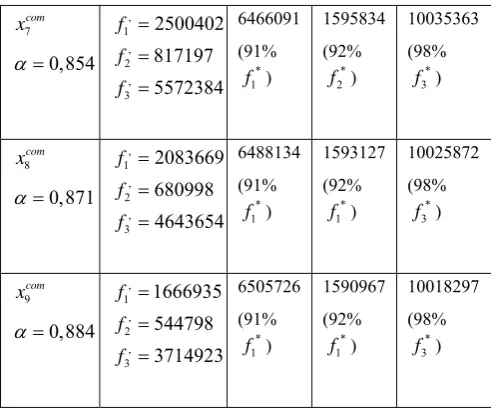
Table 8. Solution sensitivity analysis
Values of criteria functions Solution , , ,
1, ,2 3
f f f
1
f f2 f3
3 com x 0,914 α = , 1 402500 f = , 2 32775 f = , 3 312800 f = 6565953 (92% * 1 f ) 1583569 (92% * 2 f ) 9992405 (97% * 3 f ) 4 com x 0,765 α = , 1 3750603 f = , 2 1225795 f = , 3 8358576 f = 6346056 (89% * 1 f ) 1610576 (93% * 2 f ) 10087045 (98% * 3 f ) 5 com x 0,804 α = , 1 3338870 f = , 2 1089596 f = , 3 7429846 f = 6402502 (91% * 1 f ) 1603644 (93% * 2 f ) 10062742 (98% * 3 f ) 6 com x 0,833 α = , 1 2917136 f = , 2 953397 f = , 3 6501115 f = 6437665 (90% * 1 f ) 1599325 (93% * 2 f ) 10047602 (98% * 3 f ) 7 com x 0,854 α = , 1 2500402 f = , 2 817197 f = , 3 5572384 f = 6466091 (91% * 1 f ) 1595834 (92% * 2 f ) 10035363 (98% * 3 f ) 8 com x 0,871 α = , 1 2083669 f = , 2 680998 f = , 3 4643654 f = 6488134 (91% * 1 f ) 1593127 (92% * 1 f ) 10025872 (98% * 3 f ) 9 com x 0,884 α = , 1 1666935 f = , 2 544798 f = , 3 3714923 f = 6505726 (91% * 1 f ) 1590967 (92% * 1 f ) 10018297 (98% * 3 f )
With the solution x3com for the values ,
k
f we take the corresponding values of criteria functions obtained by minimization of the same criteria functions on the set of allowable solutions (nadir of criteria function values). The obtained compromise solution differs from the compromise solution x1com and
2
com
x . The greatest difference in criteria functions values is achieved in the function f1, which can
be justified by the fact that in this function the greatest difference in marginal solutions is 42%, while in the function f2the difference is 21%, and in the function f3 it
is 10%. The average achievement of the ideal point in the solution x3com is 93.67%, which is identical to the average
achievement of the ideal point in the solutionx1com. In the
solutions x4com, x5com, x6com, x7com, x8com and x9com for the
values , , , 1, 2 i 3
f f f we take the values which are by 10%, 20%, 30%, 40%, 50 % and 60% lower than their corresponding values for the solution x1com. The analysis of
the obtained compromise criteria functions values reveals an insignificant change in criteria functions values with simultaneous increase of the compromise general level value with reduction of value for , , ,
1, 2 i 3
f f f (from 0.705 to 0.884).
The performed analysis points to the low sensitivity of the obtained compromise solutions to the changes in values of , , ,
1, 2 i 3
f f f , which means that we will not be wrong if for the values of , , ,
1, 2 i 3
f f f we take any values higher than zero and lower than or equal to the smallest marginal values from the payoff table.
The application of the fuzzy multicriteria linear programming method on the real example reveals the advantages of this method in comparison to the linear programming method. The application of this method is also superior to the classical multicriteria linear programming methods because it provides the compromise solution which is closer to the ideal point.
V. CONCLUSION
manufacturing companies. The research also shows that the application of the FMLP method in solving the problem of output planning is a necessity resulting from the multiple conflicting goals of the company, so that the optimization in terms of criteria functions suitable for one goal leads to failure or inadequate achievement of other goals. The application of a suitable FMLP method leads to a compromise (non-dominated) solution, which provides acceptable values for criteria functions from the decision maker's viewpoint and thus eliminates the shortcoming.
Solving the problem of production program optimization by applying the FMLP methods we start from the assumption that the contribution of criteria functions to the achievement of company strategic goals is vague to the decision maker so that he/she cannot determine their absolute and relative importance. The decision maker is willing to accept the compromised solution offered to him/her.
From the analyst's viewpoint the use of this method does not require any additional effort in comparison to the classic MLP methods. However a developed IT system of the company is the basic assumption for the application of the FMLP method in determining the optimal production program.
In this method the decision maker takes part in selection of criteria functions and the choice of compromise solution.
Our example shows that the application of this method provides the least average deviation from the ideal point. To make a general conclusion on its applicability this method should be tested on a larger number of real examples. Its applicability should also be tested on real examples with vagueness not only in criteria functions but also in constraints.
REFERENCES
[1] Badri M.A.: „Combining the analytic hierarchy process and goal programming for global facility location-allocation problem“, International Journal of Production Economics, Vol. 62, Issue 3, 1999. p. 237 -248.
[2] Bellman, R. and Zadeh L.A.: „Decision Making in a Fuzzy Environment“, Management Science 17, 1970, B141-B164.
[3] Chakraborty, M., Chandra, M. K.: „Multicriteria decision making for optimal blending for beneficiation of coal: a fuzzy programming approach“, Omega, International Journal of Management Science, No. 33, 2005, page 413-418.
[4] Chen L.H., Tsai, F.C.: „Fuzzy Goal Programming with Different Importance and Priorities“, European Journal of Operational Research, Vol. 133, Issue 3, 2001, page 548-556.
[5] Hannan, E.L.: “On Fuzzy Goal Programming”, Decision Sciences, Vol. 12. Issue 3, 1981, Page 522-531.
[6] Lai, Y-J, Hwang C-L.: Fuzzy Multiple Objective Decision Making, Methods and Applications, Springer, 1996.
[7] Li, R. J.: Multiple objective Decision Making in a Fuzzy Environment, Ph. D. Dissertation, Department of Industrial Engineering, Kansas State University, Manhatan, 1990, KS 66506.
[8] Narasimhan, R.: “Goal Programming in a Fuzzy Environment”, Decision Sciences, Volume 11, Issue 2, 1980, Page 325-336.
[9] Onur Aköz, O, Petrovic, D.: „A Fuzzy Goal Programming Method with Imprecise Hierarchy“, European Journal of Operational Research, Vol. 181, Isuue 3,2007, page 1427-1433.
[10] T. Perić: Višekriterijsko programiranje- metode i primjene, Alca Script, Zagreb, 2008.
[11] Tamiz M., Jones D., Romero C.: „Goal programming for decision making: An overview of the current state-of-the-art“, European Journal of Operational Research 111, 1998, p. 569-581.
[12] Triantaphyllou, E.: Multicriteria decision making methods: a comparative study. Kluwer Academic Publishers, Dordrecht, 2000.