Abstract— In designing cellular manufacturing systems, cell formation is one of the most important steps which contains identification of machine cells and part families. This paper proposes a modified heuristic method for forming manufacturing cells. The proposed method includes two phases. The first phase is identification of initial machine cells by applying factor analysis to the matrix of similarity coefficients. In the second phase, an evolutionary algorithm is used to obtain the best component of machine cells and part-families. The designed method was applied to test problems from the literature in order to evaluate its performance. The results demonstrate that the designed method performs efficiently in with regard to some different criteria.
Index Terms— Cellular manufacturing, Cell formation, Factor analysis, Group technology.
I. INTRODUCTION
Numerous studies related to Group Technology (GT) and Cellular Manufacturing (CM) have been performed. Reisman et al. [1] presented a statistical review of 235 papers concentrated on GT and CM. According to their report, the literature dealing with GT/CM in early (1966-1975) appeared notably in books. The first material written about GT was that in Mitrofanov [2], and the first journal paper dealing with CM appeared in 1969 (Opitz et al., [3] ). Moreover, Reisman et al. [1] reviewed these 235 paper on a five-point scale, ranging from pure theory to practical applications.
Implementation of a CM system involves different aspects such as technology, human, organization, education, management. Unfortunately, merely a few papers corresponding to these areas have been published so far. However, the problem involved in justification of CM systems has attracted an increasing attention. Most of the researches were concentrated on the performance comparison between cellular layout and functional layout. Some researchers support the relative performance excellence of cellular layout over functional layout. Agarwal and Sarkis [4] presented a review and analysis of
S.H. H. Doulabi, H. Hojabri, S.A. Alagheband, A.A. Jaafari and H. Davoudpour are with the Department of Industrial Engineering, Amirkabir University of Technology, Tehran, Iran (e-mail: [email protected])
comparative performance researches on functional and CM layouts. Shambu and Suresh [5] focused on the performance of hybrid CM systems through a computer simulation investigation.
CM system design involves a number of research areas. In designing a cellular manufacturing system, Cell Formation (CF) is the first, most researched topic. A large number of approaches and methods have been introduced to solve this problem. Among these methods, Production Flow Analysis (PFA) is the first one which was applied by Burbidge [6]. Several review papers have been published to assort and assess various methods of CF. Among various CF models, those based on the Similarity Coefficients based Method (SCM) have more flexibility in incorporating manufacturing data into the machine-cells formation process[7].
In this paper, first, we use a mathematical approach to find the number of cells in section II.A, which was proposed by Albadawi et al. [8]. Following this, to find the best component of machine cells and part-families an evolutionary algorithm in section II.B, which was developed by Goncalves & Resende [9]. Finally, by solving some sample problems from the literature, and comparing the obtained results with the results of some referenced papers, especially [8] and [9], the performance of the proposed approach is demonstrated.
One of the advantages of the proposed approach is that we don't need to produce randomly digits to find the number of cells that has been applied in the evolutionary algorithm used by Goncalves & Resende. Determining the number of cells with a random approach increases the runtime. Moreover, this new method is superior to the analytical approach for large-scale problems in aspect of time, because it does not need to jump from one software to another.
II. THE PROPOSED APPROACH
A. Phase 1: determining initial machine cells using factor analysis
As cell formation can be considered as a dimension reduction problem in which a large number of correlated machines are grouped into a smaller set of independent cells, the proposed method uses factor analysis, which is a dimension reduction technique, to the part-machine matrix to determine the initial strong multivariate analysis tool applied to analyze interrelationships among a large number of variables to reduce their number into a smaller set of independent variables named factors.
Two-phase Approach for Solving Cell-formation
Problem in Cell Manufacturing
The input data in factor analysis must be in the form of correlations, and different methods are used to draw out a small number of factors from a sample correlation matrix. Principal Component Analysis (PCA) is the most popular method in factor analysis. In this method, all the principal components are generated in a way that they are orthogonal to each other so that the correlation between them is zero.
Using a sequenced manner with decreasing contributions to the variance, the principal components are extracted, that is, the first principal component explains most of the variation existing in the original data. Therefore, the first principal component can be considered as the best summary of the linear relationships which is present in the original data set. The second principal component can be considered as the second best representative of the linear relationships among the variables when the second principal component is orthogonal to the first. To be orthogonal to the first principal component, the second principal component must explain that proportion of the variance, which is not explained by the first principal component. Therefore, the second principal component can be defined as the linear combination of variables, which explains the maximum variance after removing the effect of the first principal component from the data. The rest of the principal components are defined similarly until all the variance in the data is accounted for. The full set of the principal components is as large as the original set of variables; however, the variances of the first few principal components are usually higher than 80% of the total variance of the original data. This implies that the data points can be precisely categorized into different clusters when projected into a space spanned by the first few principal components, called factors.
The materials on factor analysis mentioned above only features the most important characteristics of this approach. The readers are referred to the relevant literature such as that of Kleinbaum et al. [11] and Rummel [10] for detailed description of this approach.
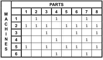
The following major steps are taken to apply factor analysis to the cell formation problem: (1) producing a similarity coefficient matrix of the machines (2) forming the initial cells applying the PCA method.These steps are explained below using an illustrative example of a simple machine cell formation problem provided by Kusiak and Cho [12].
As depicted in the table in Figure 1, the initial machine-part matrix of this problem contains six machines (labeled 1-6 in rows) and eight parts (labeled 1-8 in columns).
A1. Generation of the matrix of similarity coefficients
As mentioned earlier, the correlation matrix of the initial data set is required in order to implement factor analysis. The similarity coefficient matrix of the machines can be applied as a similarity coefficient matrix. Each element of this matrix is calculated as follow. This similarity is called Jacard similarity measure in the literature.
(
)
(1)1 1
å
å
= =
-+ = N
k
ijk jk ik
N
k ijk ij
x z y
x S
Where ij
S
: Similarity coefficient between machines i and j ijkx
: Equals 1 if operation on part k is performed on both machine i and j, otherwise 0.ik
y
: Equals 1 if operation on part k is performed on machinei, otherwise 0. jk
z
: If operation on part k is performed on machine jThis coefficient depicts maximum similarity when the two machines process the same part type, Sij =1, and maximum unlikeness when the two machines do not process the same part type, Sij =0.
The matrix of similarity coefficients shown in Figure 2 is obtained by applying Equation (1) to the initial machine-part matrix shown in Figure 1. For instance, the similarity coefficient between machines 2 and 5,
S
25, is calculated as follows:71 . 0 5 7 5
5
25= + - = S
A2. Extraction of the initial cells
Considering the machines as the original set of variables, and the similarity coefficient matrix as an acceptable estimate of the correlation matrix which accounts for the correlations between each pair of machines, we keep on using the PCA in order to group the machines into separate independent factors generating the initial cells.
The PCA method applies eigenvalue-eigenvector analysis of the similarity coefficient matrix to draw out the initial cells as shown in Equation (2)
(
S
-
I
l
)
Y
i=
0
i
=
1
,...,
P
(
2
)
where, S is an P´P similarity coefficient matrix, I is theM A C H I N E S
PARTS
1 2 3 4 5 6 7 8
1 1 1 1
2 1 1 1 1 1 1 1
3 1 1 1
4 1 1
5 1 1 1 1 1
6 1 1
Fig 1.An example of machine-part matrix
1.00 0.25 0.00 0.67 0.00 0.67 0.25 1.00 0.43 0.13 0.71 0.13 0.00 0.43 1.00 0.00 0.60 0.00 0.67 0.13 0.00 1.00 0.00 1.00 0.00 0.71 0.60 0.00 1.00 0.00 0.67 0.13 0.00 1.00 0.00 1.00
[image:2.612.90.271.628.734.2]identity matrix,
l
i s are the characteristic roots (eigenvalues), andY
is are the corresponding eigenvectors. Given in the following, Equation (3) is an eigenvalue-eigenvector equation where the termsp
l
l
l
1³
2³
...
³
are the real, nonnegative roots of the determinant polynomial of degree P.)
3
(
0
=
-
I
l
S
This system of equations is solved for
l
i, and thenY
icanbe determined, having the values of
l
i in Equation (2). It is proven that the eigenvectors computed in this way represent the unique set of P independent principal components (factors) of the data set, which maximize the variance [13]. Moreover, the elements of these eigenvectors stand for the degree of correlation between each factor and the machine, and are called the ‘factor loadings’ of the machines on the ith factor. Each of the P independent principal components indicates a cell. The corresponding eigenvalues and eigenvectors for the similarity matrix given in Figure 2 are shown in Figures 3 and 4.The user has two options in order to determine the number of cells needed to group the machines, either to determine the required number of cells in advance or to consider it as a dependent variable. In both cases, the cells must be ranked in a descending order based on the percentage of the total variance accounted for by each cell. The total variance of each cell is the sum of the variances of all machines in the cell, or the eigenvalue corresponding to that cell [13]. If the number of cells is identified by the user, then the cells with the highest eigenvalues are to be chosen. Otherwise, the cells whose eigenvalues are greater than or equal to one should be selected [14]. Both criteria assure that a high percentage of the variance is explained. The calculated eigenvalues for the matrix given in Figure 2 are ranked in a descending order in Table 1. Based on Kaiser’s criterion, only the first two cells are required to group the machines.
Table 1 illustrates the initial data for each cell. The total variance accounted for by each cell is given in the column labeled eigenvalues. The next column includes the percentage of the total variance related to each cell. The percentage of the total variance represented by each factor is used to decide on the number of cells. The last column demonstrates the cumulative percentage, which is the percentage of variance related to each cell and the cells that precede it in the table.
As shown in Table 1, nearly 79% of the total variance is related to the first two cells. The remaining four cells together, explain just 21% of the total variance. A major benefit of this method is the possibility of obtaining the optimum number of cells by considering the cells with the greater percentages of the total variance.
Table 2 indicates the initial machine-cell matrix generated by the PCA. This table includes the elements of the two chosen eigenvectors related to the highest eigenvalues. The absolute values of the elements of the eigenvectors represent the associations between the machines and the celles. For instance, based on Table 2, machine 1(m1) can be formulated as:
m
1
=
0
.
13
F
1
+
0
.
49
F
2
, so the value of the loadings that state association of machine 1 to the cells 1 and 2 are, respectively, 0.13 and 0.49 . This implies that machine 1 has a stronger relationship with cell 2 than cell 1.Consequently, machine 1 is assigned to cell 2 because it has greater absolute loading factor value. This rule is followed to assign other machines to predetermined cells.
So the initial machine set is:
(
) (
)
{
2,
3,
5,
1,
4,
6}
1
m
m
m
m
m
m
M
=
B. Phase 2: Evolutionary algorithm
The evolutionary algorithm contains an improvement procedure which is applied in an iterative scheme. Each iteration k of the procedure begins with an initial set of machine cells called
M
KINITIALl ; and generates a set of product families calledP
KINITIAL ; and a set of machine cells calledM
KFINAL , Two block-diagonal matrices can be achieved by combiningM
KINITIAL withP
KFINAL andFINAL K
M
withP
KINITIAL . Then, from these matrices, the one with the highest grouping efficacy is selected as the0.000 0 0 0 0 0
0 0.211 0 0 0 0
0 0 0.424 0 0 0
0 0 0 0.601 0 0
0 0 0 0 2.118 0
0 0 0 0 0 2.646
Fig 3.Eigenvalue matrix corresponding to the matrix shown in Fig 2.
0.000 -0.3208 0.7320 -0.3092 0.1323 0.4982 0.0000 0.5966 -0.0617 -0.5566 -0.5102 0.2649 0.0000 0.2064 0.3993 0.7148 -0.5203 0.1279 -0.7071 0.0779 -0.3047 0.1970 0.2066 0.5653 0.0000 -0.6974 -0.3394 -0.0783 -0.6051 0.1616 0.7071 0.0779 -0.3047 0.1970 0.2066 0.5653
Fig 4.Eigenvector matrix corresponding to the matrix shown in Fig 2.
Table 1. Percentage of variance associated with each cell
Cells Eigenvalues % of total variance Cumulative percentage (%)
1 2.646 44.10% 44.10%
2 2.118 35.30% 79.40%
3 0.601 10.02% 89.42%
4 0.424 7.07% 96.48%
5 0.211 3.52% 100.00%
[image:3.612.75.274.524.600.2]6 0.000 0.00% 100.00%
Table 2. Elements of two selected eigenvectors.
Machines cell 1 cell 2
1 0.1323 0.4982
2 -0.5102 0.2649
3 -0.5203 0.1279
4 0.2066 0.5653
5 -0.6051 0.1616
resulting block-diagonal matrix of the iteration k. The procedure halts if
M
KFINAL =M
KINITIAL or if the grouping efficacy of the block-diagonal matrix obtained from iterationk is not greater than the grouping efficacy of the block-diagonal matrix resulting from the earlier iteration
k-1, (for
k
³
2
). Otherwise, the procedure setsINITIAL K
M
=M
KFINAL and keeps on to iterationk
+
1
. Eachiteration k of the evolutionary algorithm contains the two following steps:
B1. Generating the set of product families:
Products are assigned to machine cells one at a time. A product is allocated to the cell that maximizes an estimate of the grouping efficacy, that is, a product is allocated to the machine cell C*, given by
ïþ
ï
ý
ü
ïî
ï
í
ì
-=
inc out c
c
N
N
N
N
C
, 1 1
, 1 1
*
arg
max
where
argmax : the argument which maximizes the expression. 1
N
:total number of 1s in matrix A . outc
N
1, : total number of 1s outside diagonal block if part isallocated to cell C. in
c
N
1, : total number of 0s inside diagonal block if part isallocated to cell C.
In this step, the algorithm produces a set of product families
P
KFINAL.B2. Generating the set of machine families
Machines are allocated to product families, one at a time. A machine is allocated to the product family which maximizes an estimate of the grouping efficacy, that is, a machine is allocated to the product family F*, given by
ïþ
ï
ý
ü
ïî
ï
í
ì
+
-=
inF out F
F
N
N
N
N
F
, 0 1
, 1 1
*
arg
max
where 1
N
:total number of 1s in matrix A . outF
N
1, : total number of 1s outside diagonal block if part isallocated to machine F. in
F
N
1, : total number of 0s inside diagonal block if part isallocated to machine F.
In this step, the local algorithm produces a new set of machine cells
M
KFINAL .B3. A numerical example of phase 2
Iteration 1:
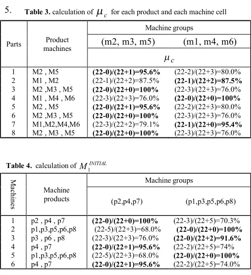
Following the example in section A, the parts are assigned to predetermined machine groups as shown in Table 3.
Table 3 indicates the value of
ïþ
ï
ý
ü
ïî
ï
í
ì
+
-=
inC Out C c
N
N
N
N
, 0 1
, 1 1
m
foreach product and each machine cell. A product is allocated to the cell with the highest value of
m
c (selected cells are bold in Table 3).If for some parts, the value of
m
c for machine groups with highestm
c values are equal, one of the machine groups is randomly selected. According to Table 3, following set is obtained.P
1INITIAL=
{
(
p
1,
p
3,
p
5,
p
6,
p
8) (
,
p
2,
p
4,
p
7)
}
Iteration 2:In this iteration based on
P
1INITIAL,M
1FINAL is generatedas shown below. Following machine groups are extracted From the Table 4 .
(
) (
)
{
2 3 5 1 4 6}
1
m
,
m
,
m
,
m
,
m
,
m
M
FINAL=
The algorithm is terminated because
M
1INITIAL=
M
1FINAL .The final machine-part matrix is reached as shown in Figure 5. Table 3. calculation of
m
c for each product and each machine cellParts machines Product
Machine groups
(m2, m3, m5) (m1, m4, m6)
c
m
1 M2 , M5 (22-0)/(22+1)=95.6% (22-2)/(22+3)=80.0% 2 M1 , M2 (22-1)/(22+2)=87.5% (22-1)/(22+2)=87.5%
3 M2 ,M3 , M5 (22-0)/(22+0)=100% (22-3)/(22+3)=76.0% 4 M1 , M4 , M6 (22-3)/(22+3)=76.0% (22-0)/(22+0)=100%
5 M2 , M5 (22-0)/(22+1)=95.6% (22-2)/(22+3)=80.0% 6 M2 ,M3 , M5 (22-0)/(22+0)=100% (22-3)/(22+3)=76.0% 7 M1,M2,M4,M6 (22-3)/(22+2)=79.1% (22-1)/(22+0)=95.4%
8 M2 , M3 , M5 (22-0)/(22+0)=100% (22-3)/(22+3)=76.0%
PARTS
M
A 1 3 5 6 8 2 4 7
C 2 1 1 1 1 1 1 0 1
H 3 0 1 0 1 1 0 0 0
I 5 1 1 1 1 1 0 0 0
N 1 0 0 0 0 0 1 1 1
E 4 0 0 0 0 0 0 1 1
S 6 0 0 0 0 0 0 1 1
Fig 5. final machine-part matrix
Table 4. calculation of MINITIAL 1
M
ac
hin
es
Machine products
Machine groups
(p2,p4,p7) (p1,p3,p5,p6,p8)
1 p2 , p4 , p7 (22-0)/(22+0)=100% (22-3)/(22+5)=70.3% 2 p1,p3,p5,p6,p8 (22-5)/(22+3)=68.0% (22-0)/(22+0)=100%
3 p3 , p6 , p8 (22-3)/(22+3)=76.0% (22-0)/(22+2)=91.6%
4 p4 , p7 (22-0)/(22+1)=95.6% (22-2)/(22+5)=74% 5 p1,p3,p5,p6,p8 (22-5)/(22+3)=68.0% (22-0)/(22+0)=100%
[image:4.612.309.556.316.586.2]III. EVALUATION OF PERFORMANCE
In this section we define four performance indicators that have been developed in literature. Each indicator should consider two criterions: the number of 1s outside the final blocks and the number of 0s inside the final block.
A. Approximation of group efficiency
This indicator is defined in last section and its higher value presents a better parts-machines component. It considers both criterions previously explained.
100
´ =
operations of
number total
elements l exceptiona of
number PE
B. Machine utilization
Machine utilization is defined by Chandrasekharan and Rajagopalan [15] as
å
== Q
k mkpk
N MU
1
Where N is number of 1s in blocks , k is number of cells ,
k
m
is number of machines in k th cell andp
k is number of parts in k th cell.C. Group efficiency
Grouping efficiency (GE) is an integrated measure, which considers both the number of exceptional elements and machine utilization. Chandrasekharan and Rajagopalan [15] defined GE as:
( )
÷ ÷ ÷ ÷
ø ö
ç ç ç ç
è æ
-´ -+ ÷ ÷ ÷ ÷
ø ö
ç ç ç ç
è æ
=
å
å
= =
Q
k k k
Q
k k k
p m N M
NE p
m N GE
1 1
1 1 a a
NE : number of exceptional elements
N
M
´
: size of part-machine matrixa
: weight coefficient (commonly is considered 0.5)IV. COMPUTATIONAL RESULTS
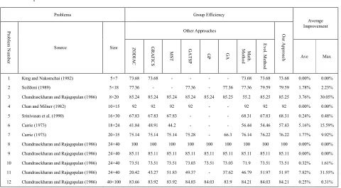
The evolutionary algorithm was tested on 12 GT instances from the literature to demonstrate the performance of the designed algorithm. The selected matrices vary in dimension5´7_40´100, and includes well-structured, as well as unstructured matrices. Table 5 is used to present the matrix sizes and their sources. We compare the grouping efficacy our algorithm with the grouping efficacies from the following eight approaches:
1)Evolutionary algorithm [9]; 2)Mathematical approach [8]; 3)ZODIAC [16]; 4)GRAFICS [17]; 5)MST [18]; 6)GATSP [19]; 7)GA [20]; 8)GP [21];
V. CONCLUSION
[image:5.612.60.540.467.732.2]In this paper a novel two-phase approach is proposed for the problem of cell formation in cellular manufacturing. The first phase which is based on factor analysis determines the number of cells. In the second phase structure of each cell including machine families and part families is obtained using an existing evolutionary algorithm in the literature. Computational results demonstrate the efficiency of the proposed algorithm.
Table 5. Experimental results
Problems Group Efficiency
Average Improvement
Pr
ob
le
m
Nu
m
ber
Source Size
Other Approaches Ou
r
A
p
pr
oa
ch
Z
O
D
IAC
G
R
A
F
ICS
M
ST
GAT
SP GP
GA Ma
th
.
M
eth
od
Evol
. M
eth
od
Ave Max
1 King and Nakomchai (1982) 5×7 73.68 73.68 - - - - 73.68 73.68 73.68 0.00% 0.00%
2 Seifdoni (1989) 5×18 77.36 - - 77.36 - 77.36 77.36 79.59 79.59 1.78% 2.23%
3 Chandrasekharan and Rajagopalan (1986) 8×20 85.24 85.24 85.24 85.24 85.24 85.25 55.2 85.25 85.25 3.76% 30.05%
4 Chan and Milner (1982) 10×15 92 92 92 92 - - 92 92 92 0.00% 0.00%
5 Srinivasan et al. (1990) 16×30 67.83 67.83 67.83 - - - 68.31 67.83 68.31 0.24% 0.48%
6 Carrie (1973) 18×24 41.84 48.91 44.2 - - - 56.44 54.46 57.43 5.16% 15.59%
7 Carrie (1973) 20×35 75.14 75.14 75.14 75.28 - 66.3 76.14 76.22 76.22 1.77% 9.92%
8 Chandrasekharan and Rajagopalan (1986) 24×40 100 100 100 100 100 100 100 100 100 0.00% 0.00%
9 Chandrasekharan and Rajagopalan (1986) 24×40 85.11 85.11 85.11 85.11 85.11 85.11 85.11 85.11 85.11 0.00% 0.00%
10 Chandrasekharan and Rajagopalan (1986) 24×40 73.51 73.51 73.51 73.03 73.51 73.03 71.9 73.51 73.51 0.32% 1.61%
11 Chandrasekharan and Rajagopalan (1986) 24×40 20.42 43.27 51.83 49.37 - 37.62 46.79 51.97 51.97 7.82% 31.55%
REFERENCES
[1] Reisman, A., Kumar, A., Motwani, J., Cheng, C.H., 1997. Cellular manufacturing: A statistical review of the literature (1965–1995). Operations Research 45, 508–520.
[2] Mitrofanov, S.P., 1966. Scientific Principles of Group Technology, Part I. National Lending Library of Science and Technology, Boston, MA. [3] Opitz, H., Eversheim, W., Wienhal, H.P., 1969. Work-piece
classification and its industrial applications. International Journal of Machine Tool Design and Research 9, 39–50.
[4] Agarwal, A., Sarkis, J., 1998. A review and analysis of comparative performance studies on functional and cellular manufacturing layouts. Computers and Industrial Engineering 34, 77–89.
[5] Shambu, G., Suresh, N.C., 2000. Performance of hybrid cellular manufacturing systems: A computer simulation investigation. European Journal of Operational Research 120, 436–458.
[6] Burbidge, J.L. (1975), The Introduction to Group Technology, John Wiley & Sons, New York, NY,
[7] Seifoddini, H., 1989a. Single linkage versus average linkage clustering in machine cells formation applications. Computers and Industrial Engineering 16, 419–426.
[8] Zahir Albadawi, Hamdi A. Bashir, Mingyuan Chen. A mathematical approach for the formation of manufacturing cells. Computers & Industrial Engineering 48 (2005) 3–21
[9] Jose´ Fernando Gonc¸alvesa, Mauricio G.C. Resende. Computers & Industrial Engineering 47 (2004) 247–273
[10] Rummel, R. J. (1988). Applied factor analysis. Evanston: Northwestern University Press.
[11] Kleinbaum, D., Kupper, L., & Muller, K. E. (1988). Applied regression analysis and other multivariable methods. California: Duxbury Press. [12] Kusiak, A., Cho, M., 1992. Similarity coefficient algorithms for solving
the group technology problem. International Journal of Production Research 30, 2633–2646.
[13] Basilevsky, A. (1994). Statistical factor analysis and related methods. Canada: Wiley.
[14] Kaiser, H. F. (1960). The application of electronic computers to factor analysis. Educational and Psychological Measurement, 20, 141–151. [15] Chandrasekharan, M. P., & Rajagopalan, R. (1986). MODROC: an
extension of rank order clustering for group technology. International Journal of Production Research, 24(5), 1221–1233.
[16] Chandrasekharan, M. P., & Rajagopalan, R. (1987). ZODIAC—An algorithm for concurrent formation of part families and machine cells. International Journal of Production Research, 25(6), 835–850. [17] Srinivasan, G., & Narendran, T. T. (1991). GRAFICS-A nonhierarchical
clustering-algorithm for group technology. International Journal of Production Research, 29(3), 463–478.
[18] Srinivasan, G., 1994. A clustering algorithm for machine cell formation in group technology using minimum spanning trees. International Journal of Production Research 32, 2149–2158.
[19] Cheng, C. H., Gupta, Y. P., Lee, W. H., & Wong, K. F. (1998). A TSP-based heuristic for forming machine groups and part families. International Journal of Production Research, 36(5), 1325–1337. [20] Onwubolu, G. C., & Mutingi, M. (2001). A genetic algorithm approach to
cellular manufacturing systems. Computers and Industrial Engineering, 39(1-2), 125–144.