AUT J. Civil Eng., 3(2) (2019) 225-232 DOI: 10.22060/ajce.2018.15303.5532
F. Hatami1*, N. Paslar2
The Effect of Dimensional Change of Boundary Elements on the Response
Modification Factor of the Steel Plate Shear Wall
1 Assistant Professor, Amirkabir University of Technology, Tehran, Iran
2 Department of Civil engineering, Islamic Azad University of Qeshm, Qeshm, Iran
ABSTRACT: During the past few decades, steel plate shear wall (SPSW) has been used as a lateral load-bearing system in building construction; however, the wall boundary conditions have been considered symmetric and identical in most of the performed projects and researches. In this paper, the Response Modification Factor of this system, when the columns are non-identical, and the effect of changing the dimensions of each boundary element have been investigated. These wall models could be seen when architectural and facility limitations are governing in the design or in the seismic retrofitting of existing structures when boundary elements especially the columns are of non-identical dimensions. Moreover, the necessity of this investigation would be important concerning the role of the Response Modification Factor in seismic design of structures. In this study, the effect of changing the dimensions of boundary elements on the Response Modification Factor of steel plate shear wall was calculated using Uang’s method and Newmark & Hall’s method. The same study has also been performed on ductility, energy absorption, and ultimate strength.
Review History:
Received: 19 November 2018 Revised: 2 January 2020 Accepted: 21 November 2018 Available Online: 21 November 2018
Keywords: Steel Plate Shear Wall Response Modification Factor Boundary Elements Ductility
Energy Absorption Non-Identical
1- Introduction
Due to their stiffness, energy absorption, and relatively more ductility than other similar systems, steel shear walls exhibit good behavior in the face of earthquake and other lateral forces. Today, it is economically proved that structures had better behave in a non-linear way against severe earthquakes. In addition, the structural elements are able to absorb and eliminate the earthquake-induced energy by means of the same behavior and ductility [1]. While our design codes are in the form of linear analyses, non-linear behavior is considered as a parameter called the Response Modification Factor (R). Response Modification Factor is, in fact, a parameter that includes the non-elastic behavior of a structure against severe earthquakes [2]. The Response Modification Factor in Iran’s 2800 code is the same correction factor used in US code, such as the IBC2000 and FEMA, or is the same correction factor used in Canadian National code NBCC 2005, which are all the same in basics but different in details [1].
Determining the precise value of this factor is of particular importance since its small values lead to designing large-scale and non-economic structures (overdesign) and its large values are considered as accepting additional levels of damages and failures in the structure [3, 4]. In 1931,
results was that the use of LYP steel reduces the forces imposed on the boundary elements of the frame compared to the standard steel [8].
In 2017, Shekastehband et al. conducted a numerical and laboratory experiment on 8 samples of steel shear walls which their infill plate was intended to be used as a hardening element or beam which was considered as a secondary column. The results of all samples were satisfactory indicating that this method could be used as another option alongside the classic steel shear wall. Their perforated model also exhibited reduced strength and ductility compared to the non-perforated one [9].
In another study conducted in 2017, they also looked at the use of low-yield-point (LYP) and high-yield-point (HYP) plates in this type of wall. The results of this study show that the use of an HYP plate can compensate for the reduction in shear capacity and energy absorption due to the non-attachment of the plate to the column in these walls [10]. Sometimes, we may encounter a frame in which the boundary components, especially the columns, are not identical on both sides of the panel due to architectural constraints or facilities, or in the context of the seismic improvement of existing structures. In this paper, besides calculating the Response Modification Factor of steel shear walls with non-uniform columns, the effects of each of the boundary components on the Response Modification Factor of these walls are also discussed.
2- Response modification factor
The response modification factor according to the fundamentals of Uang’s studies is calculated by the following method.
(1)
R =RµΩY
(2)
max
y
δ
µ
δ
=
2- 1- Ductility (μ)
Generally, ductility is interpreted as the ability of a structure to tolerate plastic deformations before fracture, that is equals to maximum story drift δmax divided by the
displacement of the structure yield δy. according to the tangential and bilinear structural curve shown in figure 1 and can be calculated as follows [1] :
eu
y
C R
C
µ = (3)
2- 1- 2- Reduction factor due to the Newmark and Hall’s ductility method
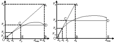
The following relations are proposed for determining Rμ for elastic-plastic systems with 1 degree of freedom according to Figure 2.
Mode 1: for hard structures or a frequency above 33 Hz (frequencies less than 0.03 seconds):
Figure 2. Bilinear curve and non-elastic behavior of a hard structure (right) and a soft structure (left) [13]
Figure 1. The actual and ideal response curve of the structure
[12]
Rμ=1 T < 0.03 sec (4) Mode 2: for hard structures or a frequency between 2 and 8 Hz (frequencies between 0.12 to 0.5 seconds):
Rμ =√2μ-1 0.12 < T <0.5 sec (5) Mode 3: for soft structures or a frequency shorter than 1 Hz (frequencies greater than 1 second):
Rμ=μ T > 1 sec (6) Where μ is the ductility factor and T is the structure frequency. Figure 2 shows the non-elastic behavior of soft and hard structures [13].
2- 2- Overstrength factor (Ω)
It is equal to the quotient of the division of the corresponding force, i.e. the overall yield limitation of a structure during the formation of the failure mechanism (Cy) by the corresponding force during the formation of the first plastic joint in the structure (Cs):
2- 1- 1- Reduction factor due to the Uang’s ductility method
Due to ductility, the building will have a capacity for hysteresis cycles and energy depletion. Due to this energy
(7) y
s
C C Ω =
2- 3- Allowable stress factor (Y)
This factor is determined in accordance with the stress of design codes (allowed load or final load) and its value is equal to the ratio of force balance during the formation of the first plastic joint (Cs) to the force balance at the allowed stress level (Cw):
(8) s
w
C Y
C
=
The value of this factor is equal to 1/4 to 1/5 [11].
3- Reference Laboratory Model
In this research, a three-story – single-bay laboratory sample proposed by Choi and Park in 2008 was used. The width and height of this sample were 2500 and 3550 mm, respectively. The infill plate of the wall was 4 mm in thickness and of the same material as SS400 steel in accordance with Korea standard. The elements of the beam and column were made of SM490 steel in accordance with the Korea standard and their sections were selected according to Table 1 (values in millimeters). The beam-to-column connection was of a flexural type and was perfectly restrained, and the bonding of the plate to the boundary elements was also possible through a fish plate, which is shown in Figure 3. The loading was of a cyclic type that was applied to the end of the upper beam according to the ATC-24 loading protocol, as shown in Figure 4. Finally, loading was terminated with the loss of resistance and buckling in the columns of the first floor. Figure 5 shows a laboratory sample after the end of loading [14].
Figure 3. Fish plate [14]
Figure 4. Sample loading chart according to ATC-24 protocol
Figure 5. Choi and Park’s laboratory sample after loading [14]
Table 1. Geometric specifications of the laboratory sample [14]
floor beam column
1st H-150×100×12×20 H-150×150×8×20
2nd H-150×100×12×20 H-150×150×8×20
3rd H-250×150×12×20 H-150×150×8×20
4- Verification
Abaqus software version 6/14-2 was used to model the pre-mentioned sample. The elements used were of the S4R type available in the software, because this type of element simulates buckling behavior of thin plate well. In the modeling process, the fish plate modeling was ignored, since it had no significant effect on the moment of inertia of the boundary elements and the final results. This method could also reduce the analysis time. The mesh size was 80 mm and the nonlinear effect of materials and geometry was considered. For loading, the ATC-24 protocol was used as a reference laboratory sample and loading was applied to the left side of the beam in the upper floor. Since no piece is ideally flat and that the middle plate might undergo surface roughness change due to various reasons, such as transportation, installation, etc., 0.1 out of every 10 primitive modes of buckling deformation were assigned to the middle plate as the initial imperfection through buckling analysis. In Figure 6, a comparison between the hysteresis curve of the laboratory sample and the software model is observed, which results in a very good approximation and modeling accuracy.
Figure 6. Comparison and validation of laboratory hysteresis
5- Definition of models
Four models were designed that differed in the type of sections of the boundary elements (beams and columns). These changes were considered based on the 100% increase
in the moment of inertia, compared to the S1 model, the details of which accord with Table 2.
In Figure 7, there is an image of the models that depicts the modified element in red.
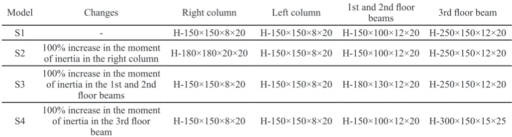
Table 2. Boundary elements and models
Model Changes Right column Left column 1st and 2nd floor beams 3rd floor beam
S1 - H-150×150×8×20 H-150×150×8×20 H-150×100×12×20 H-250×150×12×20
S2 100% increase in the moment of inertia in the right column H-180×180×20×20 H-150×150×8×20 H-150×100×12×20 H-250×150×12×20
S3 100% increase in the moment of inertia in the 1st and 2nd
floor beams H-150×150×8×20 H-150×150×8×20 H-180×130×12×20 H-250×150×12×20
S4 100% increase in the moment of inertia in the 3rd floor
beam H-150×150×8×20 H-150×150×8×20 H-150×100×12×20 H-300×150×15×25
Figure 7. S1, S2, S3, and S4 models
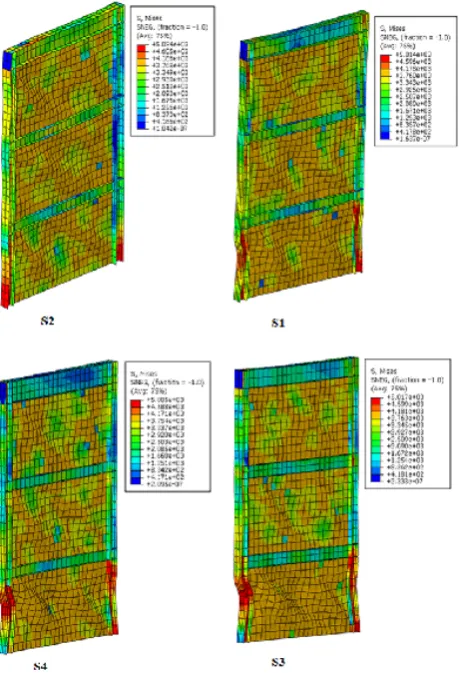
6- Results and analysis of models
The end of loading for models was considered as the first loading cycle in which the model faced with reduced resistance. The image of models after loading is shown in Figure 8. In addition, the hysteresis, pushover and bilinear curves of each model are shown in Figure 9. The pushover diagrams are plotted based on the gradual increase in displacement of each cycle (toward positive and negative loading). Also, the bilinear graph is plotted according to the conditions of the FEMA for each model, using coding in MATLAB software.
The conditions for bilinearization of the pushover diagram according to FEMA are:
1. The area under the pushover curve and the bilinear diagram is equal.
2. A bilinear diagram cuts through the pushover curve at 0.6 times its maximum value of base cutting. According to the results of loading samples in the positive and negative directions, the most critical loading mode (in two directions) was considered for each model, which showed no significant difference in the S1, S3, and S4 models. However, in the case of S2 model, given that it is asymmetric under stiffness condition and its hysteresis
curve has a significant difference when samples are loaded in positive and negative directions, the most critical mode was considered between loading in positive and negative directions. The parameters discussed are calculated and the related values are given in Table 3.
toward the stronger column, the weaker column lost its strength and reduced the sample strength. This is related to the higher stiffness and moment of inertia of the right column. In this model, the upper beam capacity was also
well-utilized. Also, the upper beam underwent buckling in the areas near the weaker column. This phenomenon is also caused by the asymmetric stiffness of the model.
Figure 8. S1, S2, S3, and S4 models
Table 3. Basic parameters and response modification factors of S1, S2, S3, and S4 models
MODEL Cy
(kN) δy (mm)
δmax
(mm) µ Energy absorption (kN.mm) Ω
Maximum
strength
(kN)
R
Uang
R Newmark and
Hall
S1 1389.29 12.07 121.14 10.03 161302.8 1.86 1517.48 21.22 11.38
S2 1405.66 10.2 98.91 9.69 141944.8 1.92 1642.51 19.67 11.56
S3 1449.07 13.76 124.75 9.06 165845.8 1.98 1626.32 20.13 11.5
S4 1428.75 12.34 124.37 10.07 167684.4 1.95 1533.86 21. 9 12
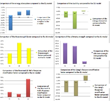
7- Comparison
The S1 model, which was Choi and Park’s laboratory sample, was considered as the reference model. Changes in parameters such as ductility, energy absorption, ultimate strength, overstrength factor, Newmark and Hall’s and Uang’s response modification factor for other models compared to this model which can be seen in Figure 10 in the form of a graph in percentage terms (positive numbers mean increasing and negative numbers mean decreasing
the desired parameter in percentage terms compared to the reference model).
8- Conclusion
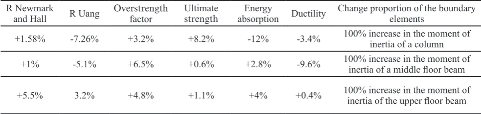
Table 4 shows the variation of the basic parameters based on the change proportion of the boundary elements in percentage terms (positive numbers mean increasing and negative numbers mean decreasing).
Table 4. Table of parameters changes relative to boundary elements
R Newmark
and Hall R Uang Overstrengthfactor Ultimate strength absorption DuctilityEnergy Change proportion of the boundary elements +1.58% -7.26% +3.2% +8.2% -12% -3.4% 100% increase in the moment of inertia of a column
+1% -5.1% +6.5% +0.6% +2.8% -9.6% 100% increase in the moment of inertia of a middle floor beam
+5.5% 3.2% +4.8% +1.1% +4% +0.4% 100% increase in the moment of inertia of the upper floor beam
The degree of ductility in the Uang’s method and the overstrength factor in the Newmark and Hall’s method play a more significant role in the calculation of the response modification factor of these methods. In the meantime, the Uang’s method also relied heavily on the structural ductility. However, in the Newmark and Hall’s method, the ductility effect has been approximated conservatively which yielded more reliable values. Also, in order to calculate the response modification factor, it is necessary to use methods that accord with the codes used in design because there are significant differences in the values of the response modification factor obtained from different methods. The response modification factor related to the steel shear wall for the S1 model, which is the same Choi and Park’s laboratory model, was calculated to be 21.22 and 11.38 by means of Uang’s and Newmark and Hall’s models, respectively.
The S2 model in which one of the columns had a 100% increase in moment of inertia, was accompanied by 3.4% and 12% decrease in the ductility and energy absorption, respectively despite an 8.2% increase in the final strength. This has led to a 7.26% reduction in response modification factor calculated by means of the Uang’s method. However, in the response modification factor of the Newmark and Hall’s method, a 3.2% increase in the overstrength factor compensated for the reduction in ductility, and as a result, the response modification factor increased by 1.58%. The response modification factor was calculated to be 19.67 by Uang’s method and 11.56 by Newark and Hall’s method. In addition, due to the asymmetric stiffness created on both sides of the panel, it is preferable to avoid such a design, as it may lead to structural torsion in larger dimensions.
The S3 model which was accompanied by a 100% increase in moment of inertia in first and second-floor beams, resulted in a 9.6% reduction in the ductility despite a slight 0.6% increase in the ultimate strength and a 2.8% increase in the energy absorption. This has led to a 5.1 % reduction in the response modification factor calculated by means of the Uang’s method. However, in the response modification factor of the Newmark and Hull’s method, a 6.5 % increase in the overstrength factor compensated for the reduction in ductility, and as a result, the response modification factor increased by 1 %. The response modification factor was calculated to be 20.13 by Uang’s method and 11.5 by Newmark and Hall’s method. The S4 model which was accompanied by a 100% increase in the moment of inertia in the upper floor beam,
resulted in an increase of 1.1% in the ultimate strength, 4% in the energy absorption, 4.8% in the overstrength and 0.4% in the ductility. This has led to a 3.2 % increase in the response modification factor by Uang’s method and a 5.5 % increase by the Newmark and Hall’s method. The response modification factor was calculated to be 21.9 by Uang’s method and 12 by Newmark and Hall’s method. According to the comparisons drawn, it seems that the upper beam plays an important role than other elements in the ductility and response modification factor. Despite the fact that only one column has been changed, the contribution of the columns to the stability and overstrength of structures cannot be overlooked. However, their direct effect on the ductility of the beams is more noticeable.
List of English Signs
R Response Modification Factor Rμ Ductility Reduction Factor Y Allowed Stress Factor Ceu Elastic design force, kN
Cy Base shear ratio at structural yield level, kN
Cs Force level in the formation of the first plastic joint, kN
Cw Design base shear ratio, kN
T the period of the structure’s rotation, S
List of Greek Signs Ω Overstrength factor μ is Ductility
Δmax Maximum displacement of the structure, mm
Δy Displacement of the structure surrender, mm
References
[1] F. Hatami, A. Ghamari, Steel and Composite Shear Wall, Amirkabir University of Technology branch, Iranian Academic Center for Education Culture & Research, Tehran, 2014.
[2] A.A. Tasnimi, A. Masoumi, Response modification factor for Reinforced concrete frames, Building & Housing Research Center (BHRC), 2006.
[4] O. Mohammadi, M. Zahrayi, Response modification factor methods and Effective parameters, in: 3th National congress of civil engineering, Islamic azad university of Sanandaj, 2011.
[5] H. Wagner, Flat sheet metal girders with very thin metal web. Part III: sheet metal girders with spars resistant to bending-the stress in uprights-diagonal tension fields, (1931).
[6] A. Rahai, F. Hatami, Evaluation of composite shear wall behavior under cyclic loadings, Journal of constructional steel research, 65(7) (2009) 1528-1537. [7] S. Sabouri-Ghomi, S. Mamazizi, Experimental
investigation on stiffened steel plate shear walls with two rectangular openings, Thin-Walled Structures, 86 (2015) 56-66.
[8] T. Zirakian, J. Zhang, Structural performance of unstiffened low yield point steel plate shear walls, Journal of Constructional Steel Research, 112 (2015) 40-53.
[9] B. Shekastehband, A.A. Azaraxsh, H. Showkati, A. Pavir, Behavior of semi-supported steel shear walls: Experimental and numerical simulations, Engineering Structures, 135 (2017) 161-176.
[10] B. Shekastehband, A. Azaraxsh, H. Showkati, Experimental and numerical study on seismic behavior of LYS and HYS steel plate shear walls connected to frame beams only, Archives of Civil and Mechanical Engineering, 17(1) (2017) 154-168. [11] I. Rasoolan, J. Hassan Abadi, Influence of height
increment on ductiliy and response modification factor of Steel plate shear walls, in: 7th National congress of civil engineering, Zahedan - Iran, 2013. [12] C.-M. Uang, Establishing R (or R w) and C d factors
for building seismic provisions, Journal of Structural Engineering, 117(1) (1991) 19-28.
[13] M. Gholhaki, A. Shiraziyan, Response modification factor by finite element method, in: 6th National congress of civil engineering, Semnan - Iran, 2011.
Please cite this article using:
F. Hatami, N. Paslar, The Effect of Dimensional Change of Boundary Elements on the Response Modification Factor of the Steel Plate Shear Wall, AUT J. Civil Eng., 3(2) (2019) 225-232.
![Figure 5. Choi and Park’s laboratory sample after loading [14]](https://thumb-us.123doks.com/thumbv2/123dok_us/10629.2000871/3.595.366.466.72.209/figure-choi-park-s-laboratory-sample-loading.webp)