Improved PSO Algorithm for Training of Neural Network in Co design Architecture

(1)

Improved PSO Algorithm for Training of Neural Network

in Co-design Architecture

Tuan Linh Dang

Hanoi University of Science and Technology Hanoi City

100000, Vietnam

Yukinobu Hoshino

Kochi University of Technology

Tosayamada, Kami City Kochi 782-8502, JAPAN

ABSTRACT

This paper proposes a new version of the standard particle swarm optimization (SPSO) algorithm to train a neural network (NN). The improved PSO, called the wPSOd−CV algorithm, is the

im-proved version of the PSOd−CV algorithm presented in a previous

study. The wPSOd−CV algorithm is introduced to solve the issue

of premature convergence of the SPSO algorithm. The proposed wPSOd−CV algorithm is used in a co-design architecture.

Exper-imental results confirmed the effectiveness of the NN trained by the wPSOd−CV algorithm when compared with the NN trained by

the SPSO algorithm and the PSOd−CV algorithm concerning the

minimum learning error and the recognition rates.

General Terms

Neural network, Particle swarm optimization, co-design architecture

Keywords

Neural network, Particle swarm optimization, FPGA, ARM, co-design architecture

1. INTRODUCTION

Today, a neural network (NN) has become a hot topic in the re-search. Many studies focus on the using of NN in different as-pects [1, 2].

The NN is invented to represent a human brain. In order to be used in the testing phase, the NN need to be trained in the training phase [3–5]. The back-propagation (BP) algorithm has investigated in previous studies. However, the PSO algorithm has shown the ad-vantages in the training of the NN compared with the using of BP to train the NN. The NN trained by the PSO algorithm had obtained higher accuracy concerning the learning error and the recognition rate than the NN trained by conventional BP algorithm [6–9]. The PSO is the algorithm based on the social behavior of a swarm. During the operation, when one particlepin the swarm found a better location than existing locations, all particles in the swarm will follow this particlep[10, 11].

The previous has investigated the NN trained by the PSO algorithm. However, normally the previous studies have used only the standard PSO (SPSO) algorithm that could stick to a local minimum to train

the NN. In this case, the NN will have a low recognition rate in the testing phase and higher learning error in the training phase. The classification tasks of the NN trained by PSO (NN-PSO) have been investigated in previous studies. However, these studies used only standard PSO (SPSO) that may easily stick to a local mini-mum during the training phase [12–14]. In this situation, the train-ing phase will be stopped immediately. This leads to a very high learning error and a low recognition rate. Therefore, it is necessary to have a PSO algorithm that solves the premature convergence of the SPSO algorithm.

In the previous research, a new architecture for co-design between hardware and software was proposed. This architecture had not only the advantages of the software side but also the advantage of the hardware side. In this architecture, the PSO is implemented in software. Thus, in the training phase, it is very easy to modify the parameters of the PSO algorithm. In addition, the PSO is not needed in the testing phase. So, the operating speed of the testing phase is not affected by the software side. On the other hand, the NN is implemented in FPGA to increase the operation speed. The NN is implemented in FPGA so that the hardware speed could be maintained [15–17].

In the previous study, an improved version of the SPSO was proposed to solve the problem of the local minimum called the PSOd−CV algorithm. Experimental results demonstrated that the PSOd−CV algorithm achieved better accuracy than the SPSO al-gorithm. This algorithm has a big jump to help the particle can be moved out of the local minimum. However, the inertia weight in the PSOd−CV algorithm is fixed. The inertia weight is the trade-off be-tween the exploration and the exploitation. With the high value of inertia weight, the algorithm will focus on the exploitation task to search in the global area. On the other hand, with the lower value of the inertia weight, the exploration task will be conducted to focus on the local area [16, 18].

The main contribution of this paper is to propose an improved version of the PSOd−CV algorithm called the wPSOd−CV algo-rithm to solve the premature convergence of the SPSO algoalgo-rithm. All three algorithms (SPSO, PSOd−CV, and wPSOd−CV) will be investigated in the experiments with several publicly recognized databases.

(2)

3 details the experiments in NN-wPSOd−CV along with results. Section 4 concludes this paper.

2. NN-wPSOd-CV 2.1 Neural network

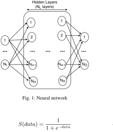
The neural network was invented to represent the human brain. Normally, the NN has three different of layers called the input layer, the output layer, and the hidden layer [3–5]. TheDnumber of weights and biases of the NN can be seen in Eq. (1).

The outputs the input layer will become the input of the hidden layer, and the output of the hidden layer will become the input of the output layer through the activation function. The activation function will fire or the output has the value of one if the input if the input is higher than threshold [3–5]. The conventional activation function is the Sigmoid function as can be seen in Eq. (2).

D= (NI+1)×NH+(NH+1)×NH×NL+(NH+1)×NO (1)

whereNI,NH, andNOare the numbers of the nodes in the input

layer, the hidden layer, and the output layer.NLis the number of

[image:2.595.101.283.292.506.2]

hidden layers as presented in Fig. 1.

Fig. 1: Neural network

S(data) = 1

1 +e−data (2)

wheredatais the input data of the Sigmoid function, andS(data)

is the output of the activation function.

2.2 Neural network trained by standard PSO

To be used, the NN needs to be trained. A famous training method is the back-propagation (BP) algorithm. However, the previous paper mentioned the accuracy advantage of the NN trained by PSO when compared with the NN trained by BP algorithm [6–9]. The previous paper proposed a framework for the co-design of the NN trained by PSO algorithm [15–17].

The original of the SPSO is from social behaviors. When one par-ticle in the swarm found a better position than the current best po-sition, the new best position is updated. In addition, other particles in the swarm have the tendency to move to the position of new best position [10, 11].

The operation of the NN trained by the SPSO (NN-PSO) algorithm is based on the operations of the SPSO [10, 11]. The NN-PSO can be detailed as follows.

(1) The weights and the biases of the neural network are encoded into the PSO particles. The dimension of one particle equals the number of weights and biases of the neural network. In the initial phase at timet, the positions of all particles are ran-domly generated. Thus it has:

—Position of particlepisxp(t)

—Velocity of particlepisvp(t)

—Best personal position of particlepisx−P bestp(t)

—Best global position of all particles in the swarm is

x−Gbest(t)

—Fitness value for the best personal position of particlepis

P bestp(t)

—Fitness value for the best global position of all particles is

Gbest(t)

(2) At next time t+ 1, calculate the new velocity according to Eq. (3)

vp(t+ 1) =w×vp(t) +c1×r1(x−P bestp(t)−xp(t))

+c2×r2(x−Gbest(t)−xp(t))

(3)

where w is inertia weight,c1andc2are coefficients.

(3) The new position at timet+ 1 is also evaluated based on Eq. (4). Each position of a particle is considered as one set of potential parameters for the NN. When the particle has a new position, the corresponding weights and the biases of the NN are also changed. Each particle hasDdimensions.D is also the size of the NN that can be calculated by Eq. (1).

xp(t+ 1) =xp(t) +vp(t+ 1) (4)

(4) The new fitness valuesP bestp(t+ 1)andGbest(t+ 1)at time

t+ 1are calculated. The calculation of new fitness values uses the output data from the NN. The parameters of the NN come from the position of the PSO particles. The output data from NN will be evaluated with the labeled data by mean squared error function as seen in Eq. (5).

The minimum learning error of each particle (P best) and the global minimum learning error (Gbest) of all particles are cal-culated

fi=

1 T

T

X

j=1

(labeledj(k)−outputij(k))2 (5)

whereT is the number of training samples,labeled(k)and

output(k)are thekth_{component of the particle}_i_{in the}

la-beled data and the output data of the NN. (5) the stopping condition is checked.

—If the condition is satisfied, the training phase of the NN trained by PSO is stopped, the finalGbestis found. Hence, the final position x−Gbest(t) corresponds to the final

Gbestis also found. This final position corresponds to the weights and biases of the NN after the training phase. —If the condition is not satisfied. A new iteration of the

train-ing will be conducted. The traintrain-ing phase return to step 2.

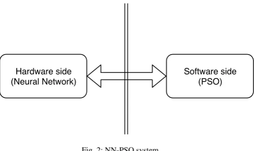
2.3 Hardware implementation of the NN-SPSO

(3)

Hardware side (Neural Network)

[image:3.595.55.305.66.214.2]

Software side (PSO)

Fig. 2: NN-PSO system

The PSO algorithm is implemented on the software side. The PSO is only used in the training phase to determine the weights and the biases of the NN. In addition, during the training, the software-based PSO may easy to change the parameter such as the inertia weightw, the coefficientsc1, c2, or even the new PSO algorithm can be used with the need to redesign or rebuild the FPGA side. The NN is coded on the hardware side using SystemVerilog pro-gramming language to take the speed advantage of the hardware-based program when compared with the conventional software-based program. The hardware-software-based normally has a higher operat-ing speed thanks to the parallelism. The NN is the only component used in the testing phase, therefore the speed of the software-based algorithm does not affect the system.

In the training phase, theDweights and biases of the NN are en-coded in the PSO particles. Each PSO particle is aD-dimensional vector. As presented,Dis calculated according to Eq. (1). The posi-tion of each particle corresponds to a potential set of weights and bi-ases for the NN. The PSO algorithm is conducted to find theGbest

fitness value and also the corresponding position of theGbest. The found position of the particle is the trained weights and biases of the NN. These trained parameters are sent to the hardware side (NN module). The NN keeps the trained weights and biases and uses these parameters in the testing phase.

2.4 Neural network trained by improved particle swarm optimization

2.4.1 Linearly decreasing inertia weight. The linearly decreas-ing inertia weight was presented to improve the performance of the standard PSO algorithm by using a strategy for weight control. This algorithm reduces the weights by iterations as can be shown in equation 6. The linearly decreasing inertia weight strategy has two tasks called the exploration and the exploitation, respectively. The particles in the swarm do a global search at the beginning (the exploitation). When inertia weightwis small, the particles conduct the exploration. This inertia weight control has the possibility to search and find the local solutions [19].

w=wmax−

wmax−wmin

Niteration

×iteration (6)

where Niteration is the number of iterations, w is the inertia

weight.

2.4.2 Particle swarm optimization with control of velocity and in-ertia weight. As described in the previous section, the PSOd−CV algorithm always has the big jumps to explore a wide area in the

jumping phase. Therefore, this algorithm has the possibility to skip local solutions in high dimensional problems. In the PSOd−CV al-gorithm, the value of the inertia weightwis fixed. However, the control of this weight has an impact on the PSOd−CV algorithm. The inertia weight control is the trade-off between the exploration and the exploitation. With a significant value ofw, the PSO al-gorithm tends to search the global area. On the other hand, with a small value ofw, the PSO algorithm tends to focus on the local area. A famous technique for weight control is the linear decreasing strategy. This strategy focuses on the exploitation task at the begin-ning of the algorithm. After that, the exploration job is addressed to search in the local area [19]. This strategy has the chances to find local solutions.

This paper proposes the PSO with control of velocity and iner-tia weight algorithm (wPSOd−CV algorithm). This algorithm is the combination of the PSOd−CV algorithm and the inertia strat-egy. Thus, this algorithm may overcome the disadvantage of the PSOd−CV algorithm. The wPSOd−CV algorithm is given in equa-tion (7).

vp(t+ 1) =wmax−

wmax−wmin

Nite

×ite×vp(t)

+c1×(x−P bestp(t)−xp(t))

+c2×(x−Gbest(t)−xp(t)) +

c3×r

(vp(t))2

(7)

whereNiteis the number of iterations,iteis the current iteration,

c1, c2, c3are the coefficients, r is the random number.

3. EXPERIMENTS

The experiments were conducted with the DE1-SoC development board provided by Altera [21]. The Hardware based NN is coded in SystemVerilog programming language while the PSO algorithms were implemented in ARM processor attached to the DE1-SoC board. The connection between the hardware side and the software side was done by direct memory access (DMA) mechanism. The experiments investigated three different PSO algorithms which were SPSO, PSOd−CV presented in the previous research, and the proposed wPSOd−CV algorithm.

Based on the tests, a suitable set of parameters for all three algo-rithms was as follows.

(1) w= 0.7,c1= 0.5,c2= 0.3 in the standard PSO algorithm. (2) w= 0.7,c1= 0.5,c2= 0.3,c3= 0.00001 in the PSOd−CV

algorithm.

(3) wmax= 0.7,wmin= 0.3,c1= 0.5,c2= 0.3,c3= 0.00001 in

the wPSOd−CV algorithm.

Four different databases were used in the experiments called XOR problem, Iris dataset, Balance-scale dataset, and Credit approval dataset.

3.1 XOR problem

The first experiment was conducted with the XOR problem, a non-linear problem. The configurations of the NN were two input nodes, six hidden nodes, and four output nodes. The parameters of this ex-periment were 50 particles, 150 iterations.

(4)

0.0 0.2 0.4 0.6

0 50 100 150

Number of iterations

Gbest

Algorithm wPSOd_CV PSOd_CV Standard PSO

Fig. 3: The reduction ofGbest

[image:4.595.76.273.65.204.2]

be subtle. For example, theGbestof the standard PSO was 0.323 in iteration 17 and this number reduced to 0.321 in iteration 38. The finalGbestafter 150 iterations of the standard PSO algorithm was 0.278, the PSOd−CV algorithm was 0.195, and the wPSOd−CV algorithm was 0.005. The wPSOd−CV algorithm obtained better performance than the other two algorithms in this experiment. The results of the co-design program were observed in the PuTTY software. For example, the results of the NN trained by the wPSOd−CV algorithm with the XOR problem were shown in Fig. 4. For reference, Table I shows the training data.

[image:4.595.59.289.345.433.2]

Fig. 4: The output in PuTTY software

Table I. : The training data of the XOR problem

Input Output1 Ouput2 Outpu3 Output4

1 1 0 0 0 1

1 0 0 0 1 0

0 1 0 1 0 0

0 0 1 0 0 0

3.2 Iris dataset

In the previous experiment, the NN was capable of solving the XOR problem. It is needed to investigate the operation of the pro-posed co-design with a classification dataset comes from daily life. However, this research uses Cyclone V which has the lowest num-ber of resources in the Altera device family [20]. Thus, the Iris dataset was chosen. This dataset has three different classes called Setosa, Versicolour, and Virginica. Each class has 50 samples. Each sample has four different attributes (the sepal length, the sepal width, the petal length, and the petal width) [22].

The NN in this experiment had four input nodes (for four at-tributes), three output nodes (for three classes), ten hidden nodes, and two hidden layers. The configuration was 4-10-10-3.

The Iris dataset was separated into two sets. The bigger set had 105 samples (each class had 35 samples). On the other hand, the smaller set had 45 samples (each class had 15 samples).

Several experiments were conducted to investigate the operation of three algorithms in different situations. Therefore, various values for the number of training data, the number of iterations and the number of particles were chosen.

In the first scenario, the bigger set was used as the training data and the other set was considered as the testing data. The number of particles was modified from a small value to a big value.

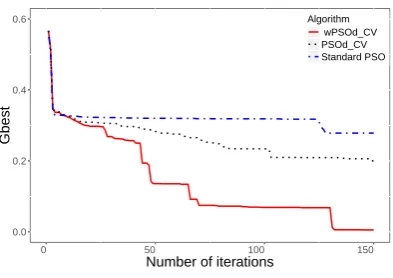
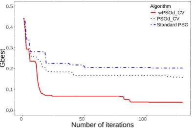
Fig. 5 and Fig. 6 describe the reduction ofGbest, the global min-imum value of learning error. In these experiments, the number of particles was 20, and the numbers of iterations were 100 and 340. In both experiments, the finalGbestof the wPSOd−CV al-gorithm decreased to the lowest value (0.1774 in the case of 100 iterations and 0.0510 in the case of 340 iterations). The finalGbest

of the PSOd−CV algorithm was 0.1944 (100 iterations) and 0.0883 (340 iterations). The finalGbestof the standard PSO algorithm was 0.2012 in both scenarios. Concerning the recognition rate, the wPSOd−CV also obtained a higher recognition rate (77.78% in 100 iterations and 93.33% in 340 iterations) than the PSOd−CV al-gorithm (66.67% in 100 iterations and 93.33% in 340 iterations) and the standard PSO algorithm (only 66.67%). Therefore, the wPSOd−CV algorithm may obtain a lowGbestand a high recog-nition rate even with the small number of particles.

0.0 0.1 0.2 0.3 0.4 0.5

0 25 50 75 100

Gbest

[image:4.595.337.539.357.491.2]

Fig. 5: The reduction ofGbestwhenP= 20 particles, 100 iterations

0.0 0.1 0.2 0.3 0.4 0.5

0 100 200 300

Gbest

[image:4.595.85.262.500.564.2]

[image:4.595.336.537.537.669.2]

(5)

In the next experiments, the number of particles was changed to increase the recognition rate and to reduce the finalGbest. Fig. 7 presents theGbestin all three algorithms when the number of particlesP= 42. Table II shows the finalGbestand the recognition rate whenP= 100. As seen in Table II and Fig. 7, the wPSOd−CV algorithm had a lowerGbestand also had a better recognition rate than the PSOd−CV algorithm and the standard PSO algorithm.

0.0 0.1 0.2 0.3 0.4 0.5

0 50 100

Gbest

[image:5.595.337.538.67.202.2]

[image:5.595.76.276.152.283.2]

Fig. 7: The reduction ofGbestwhenP= 42 particles

Table II. : The results of three different PSO algorithms whenP = 100 particles

Number of iterations Algorithm Gbest Recognition rate

100 Standard PSO 0.0669 93.33%

PSOd−CV 0.0541 95.56%

wPSOd−CV 0.0457 100.00%

230 Standard PSO 0.0577 97.78%

PSOd−CV 0.0368 100.00%

wPSOd−CV 0.0210 100.00%

[image:5.595.333.538.318.450.2]

Another experiment was conducted to investigate the operation of the proposed system with a small number of training data. In this experiment, the smaller set (45 samples) was used as the training samples. The number of particles and the number of iterations were chosen randomly (P= 80 particles, 40 iterations).

Fig. 8 illustrates theGbestof three algorithms. The wPSOd−CV al-gorithm still produced better results than the PSOd−CV alal-gorithm and the standard PSO algorithm (the finalGbestand the recogni-tion rate of wPSOd−CV were 0.0277 and 95.28%, respectively). The results of the PSOd−CV algorithm were Gbest = 0.0284, recognition rate = 94.29%. The results of the standard PSO algo-rithm wereGbest= 0.1698, the recognition rate = 76.19%.

3.3 Balance-scale dataset

Another dataset, called Balance-scale dataset, was also tested in order to investigate the operation of the NN trained by three dif-ferent PSO algorithms in difdif-ferent situations. This dataset has the same number of classes and attributes with the Iris dataset. Thus, the configuration of the NN in this experiment was similar to the configuration of the NN in the Iris experiment (4-10-10-3). Three attributes of this dataset are “right state”, “left state”, and “balance state”, respectively. The names of four attributes are “left weight”,

0.0 0.1 0.2 0.3 0.4 0.5

0 10 20 30 40

Gbest

Fig. 8: The reduction ofGbestwith 45 samples as training data

“left distance”, “right weight”, “right distance”. The values of the attributes are from one to five.

The Balance-scale dataset was also divided randomly into two sets. The first set which had 200 samples was considered as the training set. On the other hand, the second set that contains 60 samples was selected as the testing set.

The configurations for the PSO were 200 iterations, 50 particles.

0.0 0.1 0.2 0.3

0 50 100 150 200

Gbest

[image:5.595.55.291.369.451.2]

Fig. 9: The reduction ofGbestin the Balance-scale dataset experiment

Table III. : The results of the experiment with the Balance-scale dataset

Algorithm Gbest Recognition rate

Standard PSO 0.2689 81.67%

PSOd−CV 0.1298 85.00%

wPSOd−CV 0.0077 90.00%

Fig. 9 and Table III demonstrate the accuracy results of the exper-iment with 50 particles, 200 iterations. The wPSOd−CV algorithm also obtained the best recognition rate among the three algorithms.

3.4 Credit approval dataset

[image:5.595.354.514.521.573.2]

(6)

of the attributes are not disclosed [22]. The configuration of the NN was 14-24-2.

The first experiment investigated the situation when the numbers of samples from each class were equal. For example, 175 samples from class 1 and 175 samples from class 2 were selected randomly as 350 training samples. The testing samples 125 data from set 1 and 125 data from set 2.

To investigate different cases, the number of iterations and particles were modified from 10 particles, 50 iterations in scenario 1 to 50 particles, 100 iterations in scenario 2.

[image:6.595.335.538.68.201.2]

The reductions of the minimum learning errorGbestin the first scenario and second scenario are shown in Fig. 10, and Fig. 11, respectively. The results which are given in table IV demonstrated the performance of the proposed wPSOd−CV algorithm for train-ing the FPGA-based NN in the co-design architecture.

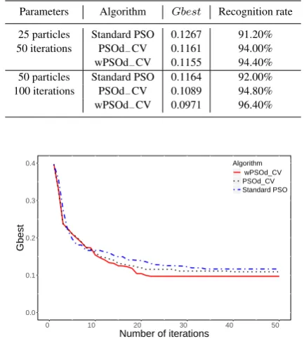
Table IV. : Credit approval dataset, 350 training samples, 250 testing sam-ples

Parameters Algorithm Gbest Recognition rate

25 particles Standard PSO 0.1267 91.20%

50 iterations PSOd−CV 0.1161 94.00%

wPSOd−CV 0.1155 94.40%

50 particles Standard PSO 0.1164 92.00%

100 iterations PSOd−CV 0.1089 94.80%

wPSOd−CV 0.0971 96.40%

0.0 0.1 0.2 0.3 0.4

0 10 20 30 40 50

Gbest

[image:6.595.334.538.248.381.2]

Fig. 10: The reduction ofGbestwith 350 training samples, 25 particles, 50 iterations

The second experiment used the training set and testing set that did not have an equal number of samples from each class. For exam-ple, 272 samples of set 1 and 229 samples of set 2 were randomly included in the training set. The testing set had 190 samples. The number of particles was 50, and the number of iterations was 100. The reduction ofGbestis presented in Fig. 12. The finalGbestof the wPSOd−CV algorithm decreased to the lowest value (0.1324) while the finalGbestof the PSOd−CV algorithm was 0.1332, and the finalGbestof the standard PSO algorithm was 0.1421. The recognition rates of the NN trained by these three algorithms are illustrated in table V. The wPSOd−CV algorithm also obtained the highest recognition rate (88.95%).

The experimental results show that the proposed wPSOd−CV al-gorithm obtained the best performance among the three alal-gorithms (wPSOd−CV, PSOd−CV, and standard PSO).

0.0 0.1 0.2 0.3 0.4

0 25 50 75 100

Gbest

0.0 0.1 0.2 0.3

0 25 50 75 100

Gbest

[image:6.595.64.281.258.501.2]

Table V. : Credit approval dataset, 500 training samples, 190 testing samples

Algorithm Gbest Recognition rate

Standard PSO 0.1421 83.65%

PSOd−CV 0.1332 86.84%

wPSOd−CV 0.1324 88.95%

4. CONCLUSION

This paper presents the new PSO algorithm called the wPSOd−CV algorithm which is the improved version of the PSOd−CV algo-rithm presented in the previous paper. In light of the evidence, experimental results confirmed that the neural network trained by PSO algorithms (SPSO, PSOd−CV, wPSOd−CV) was successfully developed. The results also stated that the proposed wPSOd−CV algorithm obtained higher accuracy concerning the learning errors

Gbestand the recognition rates than two other PSO algorithms with different datasets and different PSO parameters (number of it-erations, number of particles). The proposed PSO algorithm could help the training phase of the NN out of the local minimum to in-crease the training efficiency.

[image:6.595.353.514.451.504.2]

(7)

investigate the using of the proposed NN-wPSOd−CV in real-life applications.

5. REFERENCES

[1] P.M. Ravdin, G. M. Clark GM, A practical application of neural network analysis for predicting outcome of individ-ual breast cancer patients,Breast Cancer Research and Treat-ment, vol. 22, no. 3, pp. 285-293, 1992

[2] A. E. Celik, Y. Karatepe, Evaluating and forecasting bank-ing crises through neural network models: An application for Turkish banking sector,Expert Systems with Applicationsvol. 33, no. 4, pp. 809-815, 2007

[3] S. Haykin,Neural networks and learning machines, 3rd edn, Prentice Hall, 2008

[4] R. H. Nielsen, Theory of the backpropagation neural network, In processing of the international conference on neural net-works, pp. 693-605, 1989

[5] R. Rojas, Neural networks - a systematic introduction, Springer-Verlag, 1996

[6] J. R. Zhang, J. Zhang, T. M. Lok. M. R. Lyu, A hybrid particle swarm optimizationback-propagation algorithm for feedfor-ward neural network training,Applied mathematics and com-putation, vol. 185, pp. 10261037, 2007

[7] Z.A. Bashir, M.E. El-Hawary, Applying Wavelets to Short-Term Load Forecasting Using PSO-Based Neural Networks, IEEE transactions on power systems, vol. 46, pp. 268-275, 2016

[8] A. Suresh, K. V. Harish, N. Radhika, Particle Swarm Opti-mization over Back Propagation Neural Network for Length of Stay Prediction,In processing of the international confer-ence on information and communication technologies, vol. 24, no.1, pp. 20-27, 2009

[9] V. G. Gudise, G. K. Venayagamoorthy, Comparison of parti-cle swarm optimization and backpropagation as training al-gorithms for neural networks, In processing of 2003 IEEE swarm intelligence symposium, pp. 110-117, 2003

[10] J. Kennedy, R. Eberhart, Particle swarm optimization,In pro-cessing of the IEEE international conference on neural net-works, vol. 4, pp.1942-1948, 1995

[11] R. Eberhart, Y. Shi, Particle swarm optimization: develop-ments, applications and resources,In processing of the 2001 IEEE international conference on congress on evolutionary computation, vol. 1, pp. 81-86, 2001

[12] R. Mendes, et al., Particle swarms for feedforward neural net-work training,In processing of the IEEE international joint conference on neural networks, vol.2, pp.1895-1899, 2002 [13] K. W. Chau, Application of a PSO-based neural network in

analysis of outcomes of construction claims.Automation in construction, vol. 16, no. 5, 642-646, 2007

[14] G. Montavon, G. B. Orr, K. R. MullerNeural networks: tricks of the trade, 2nd edn, Springer, 2012

[15] T. L. Dang, Y. Hoshino, Hardware/Software Co-design for a Neural Network Trained by Particle Swarm Optimization Al-gorithm,Neural Processing Letters, pp. 1-25, 2018

[16] T. L. Dang, C. Thang, Y. Hoshino, Hybrid hardware-software architecture for neural networks trained by improved pso al-gorithm,ICIC Expree Letters, pp. 565-574, 2017

[17] T. L. Dang, Y. Hoshino, An-FPGA based classification system by using a neural network and an improved particle swarm optimization algorithm,In processing of the 2016 Joint 8th International Conference on Soft Computing and Intelligent Systems (SCIS) and 17th International Symposium on Ad-vanced Intelligent Systems, pp.97-102, 2016

[18] Y. Hoshino, H. Takimoto, PSO training of the neural network application for a controller of the line tracing car,In: Proceed-ings of the IEEE International Conference on Fuzzy Systems, pp.1-8, 2012

[19] Y. Shi. R.Eberhart R, A modified particle swarm optimizer,In Proceedings of 1998 IEEE International Conference on Evo-lutionary Computation, pp 69-73, 1998

[20] Altera company, SoC product brochure.

https://www.altera.com/products/soc/overview.html, ac-cessed 07 February 2019

[21] Terasic company, DE1-SoC user manual,

http://de1-soc.terasic.com, accessed 07 February 2019 [22] M Lichman, UCI Machine Learning Repository,