Simplified models for heating system optimisation
using the thermal–electrical analogy
O. M. Tate, D. Cheneler and C. J. Taylor Engineering Department, Lancaster University, UK
Emails: [email protected], [email protected], [email protected]
Abstract—The well-known electrical analogy for thermal mod-elling is based on the observation that Fourier’s equation for one dimensional heat transfer takes the same form as Ohm’s law. This provides a system for creating and resolving complex heat transfer problems using an established set of physically–based laws. The present article illustrates the concept for adjacent rooms in a modern university building, and investigates some of the modelling issues involved. The electrical analogy is chosen so that the models can be extended and used for future research into demand–side control of multiple buildings on the university network, requiring a fast computation time. For illustrative pur-poses, the present article is limited to a relatively straightforward two–room system, for which the modelling equations are conve-niently represented and solved using MATLAB–SIMULINK. The coefficients of this model are estimated from data using standard nonlinear optimisation tools. For comparison, the article also develops an equivalent multiple–input Transfer Function form of the model. Finally, suggestions are made for the inclusion of occupancy estimates in the model.
Index Terms—thermal modelling; building occupancy; micro-climate; transfer function; electrical analogy
I. INTRODUCTION
The research behind this article ultimately concerns control system robustness and overall system optimisation, for the regulation of temperatures in buildings that are linked to a controllable external heating supply network. This is the case, for example, with the Lancaster University campus, for which a central energy centre supplies the hot water used to heat around 50% of the buildings. More generally, Heating, Ventilation and Air Conditioning (HVAC) systems have high energy requirements, hence there is considerable interest in the development of improved optimisation tools, micro–climate control algorithms and energy management systems. Selected examples of such research include [1]–[7].
In this regard, numerous approaches for modelling heat transfer phenomena and energy use have been developed over the past few decades. The models obtained are commonly categorised into physically–based models and models that are statistically identified from data [8]. Within this context, various zonal and multi–zone approaches exist. Of particular relevance to the present article, these include thermal models constructed using an analogy with electrical systems. An early reference by Paschkis and Baker [9] describes how components of a building are considered to store or resist heat flows, equivalent to capacitors and resistors in electrical systems [10]. Research on the concept includes consideration of multiple layered walls [11], heat exchanger networks [12],
global building models [13], parameter estimation, optimal model order identification and model reduction [14]–[16].
Following a brief overview of the methodology (section II), the present article illustrates the concept for two adjacent rooms in a modern university building (sections III and IV), and discusses some of the modelling issues involved. The electrical analogy is chosen so that the models obtained can be quickly extended and used for future research into demand–side control [4] of multiple buildings on the uni-versity network, requiring a fast computation time for energy optimisation purposes. With this objective in mind, the model should be simple to construct and implement, initially using readily available physical parameters, such as room dimen-sions and estimates of thermal resistance. However, since the University’s Building Management System (BMS) includes comprehensive data collection for many parts of the campus, temperature measurements are exploited where possible to optimise the model coefficients (section V).
Finally, the model is represented using an alternative multiple–input Transfer Function form (section VI). By gen-eralising and exploiting this structure, the model is identified and estimated directly from the BMS data set and subsequently interpreted in terms of the electrical analogy, representing an example of data–based mechanistic (DBM) analysis [1]. How-ever, this approach raises identifiability challenges because of direct and indirect associations between the inputs and outputs of the model. Analysis of the initial model highlights another limitation, namely the lack of a time–varying internal heat source to represent changing occupancy rates. As a result, the model is extended to include novel occupancy estimation using data from both Wi–Fi usage and CO2 levels.
II. METHODOLOGY
TABLE I
ANALOGOUS ELECTRICAL AND THERMAL PARAMETERS.
Thermal Electrical
Symbol Parameter Symbol Parameter
∆T Temperature Difference ∆V Voltage Difference
q Heat Flow I Current
C Heat Capacity C Capacitance
R Thermal Resistance R Resistance
TABLE II NOTATION AND UNITS
Symbol Brief explanation Units
T1 Temperature of Room One K
T2 Temperature of Room Two K
T1s Supply Air Temperature to Room One K
T2s Supply Air Temperature to Room One K
TA Ambient (Outside) Air Temperature K
TE External (Surrounding) Air Temperature K
R1 Thermal Resistance Between Room One and Surroundings K/W R2 Thermal Resistance Between Room Two and Surroundings K/W R12 Thermal Resistance Between Rooms One and Two K/W C1 Thermal Capacitance of Room One J/K C2 Thermal Capacitance of Room Two J/K
q1 Heat Flow into Room One W
q2 Heat Flow into Room Two W
˙
m1 Mass Flow Rate into Room One kg/s
˙
m2 Mass Flow Rate into Room Two kg/s
U1 Internal Heat Generation in Room One W U2 Internal Heat Generation in Room Two W cp Specific Heat Capacity of Air J/Kkg
ρ Air Density kg/m3
L Wall Thickness m
k Thermal Conductivity W/mK
A Wall Area m2
V Room Volume m3
Q Flow Rate m3/s
P Power level
n Number of Vents
air gaps, as a system with three resistors and one capacitor (denoted 3R1C). However, as a greater number of zones are modelled concurrently, the network diagrams can become very large. In this case, programs such as TRNSYS [17] have been used to collate the models. Since the present article is limited to a two–room system, the modelling equations are conve-niently represented and solved using MATLAB–SIMULINK. Table II summarises the notation and associated units utilised throughout the article. Selected model coefficients are esti-mated from data using fminsearch. The Transfer Function form is estimated using Refined–Instrumental Variable (RIV) methods in the CAPTAIN Toolbox [18].
III. CASE STUDY
Lancaster University campus has several recently con-structed buildings fully instrumented with a range of sensors and actuators, and seems well suited for research into the optimisation of energy efficiency because of the associated BMS data collection capacity. Charles Carter Building, for example, is a freestanding building lying in the south part of the university’s main campus. Named after the founding Vice-Chancellor, the architects integrated various energy–reducing features into the building design, which achieved a BREEAM Excellent rating. The south elevation is designed to shade the building while the concrete roof protects the top floor from
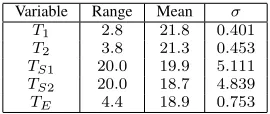
TABLE III
TEMPERATURE RANGE,MEAN AND VARIANCE.
Variable Range Mean σ
T1 2.8 21.8 0.401
T2 3.8 21.3 0.453
TS1 20.0 19.9 5.111 TS2 20.0 18.7 4.839 TE 4.4 18.9 0.753
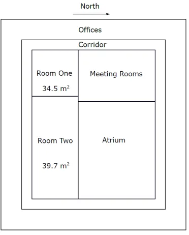
heating up in the sun. The building footprint is 33 m by 36 m with four floors (A–D). Internally the building is laid out around a central atrium that is open from the floor to the roof. Surrounding this area are lecture theatres, offices, meeting rooms and break-out spaces. Detailed micro-climate data are collected by the BMS every 10 minutes including, for example, the supply and return air temperatures for various rooms, ventilation power levels and HVAC set points.
For illustrative purposes in the present article, data from September 2017 are selected for analysis. The data and asso-ciated model focus on two research student office spaces on C floor, termed room one and room two in this article. The corner of room one meets the north–east corner of the central atrium, while room two adjoins room one, stretching along the south side of the atrium, as shown in Fig. 1. For context, Table III provides some descriptive statistics for the first week of September 2017, while Fig. 2 show typical temperatures in each room, denoted T1 and T2, as well as the associated
air supply temperatures, Ts1 and Ts2, and the surrounding
‘external’ temperatureTE(taken from adjacent meeting rooms
and assumed to be representative).
For the data under consideration here, the supply tempera-tures are reduced during the working day in order to maintain the room set points, as illustrated by Fig. 2. The supply temperatures are constant during the weekend. This pattern is repeated during the first 25 days of the month, during which time the rooms are generally warmer than the supply and ambient temperatures. By contrast, the right hand side of Fig. 2 shows that the supply temperatures are significantly higher during the last few days of September, although there is no obvious change in the outside temperature profile to explain this. For the model optimisation example considered later, the first two weeks of September 2017 are used for estimation purposes and the final two weeks for validation. This approach ignores the changing dynamics noted above and clearly requires more research. Finally, it is clear that room two is consistently a little colder than room one, and suffers greater variation in temperature, which is likely to be due to its position next to the atrium, with the associated heat losses.
IV. MODEL FORMULATION
Fig. 1. Approximate layout of the Charles Carter Building, C-floor.
0 2 4 6 8 10 12 14 16 18 20 22 24 26 28 20
22 24
oC
room 2 room 1
0 2 4 6 8 10 12 14 16 18 20 22 24 26 28 15
20 25 30
oC
supply 2 supply 1
0 2 4 6 8 10 12 14 16 18 20 22 24 26 28 day of the month
10 20
oC
[image:3.612.345.553.100.165.2]ambient outside
Fig. 2. Room, supply and external temperatures for September 2017.
rooms. As the intention is to formulate a simple model, a 1R1C system is initially assumed for each room. The heat balance diagram and equivalent RC circuits are illustrated in Fig. 3. Hence, assuming two rooms of internal temperature T1 and T2, and heat capacityC1andC2respectively, are joined by a
wall of resistance R12, then the heat balance equations yield,
q1=C1 dT1
dt +
T1−T2 R12
+T1−TE
R1
(1)
q2=C2 dT2
dt +
T2−T1 R12
+T2−TE
R2
(2)
where R1 and R2 represent the thermal resistance between
each room and the surrounding temperatureTE, and in which
the rooms are supplied with heat flows q1 andq2. The latter
are not directly measured hence are represented in the model as qi= ˙micp(Tsi−Ti)wherei= 1,2. Finally, equations (1)
and (2) are re-arranged to isolate the room temperatures, dT1
dt =
1
C1
q1+
T2−T1 R12
+TE−T1
R1
(3)
dT2 dt =
1
C2
q2+
T1−T2 R12
+TE−T2
R2
(4)
Equations (3) and (4) represent a system with two coupled temperature output variables of interest and three input signals i.e.Ts1,Ts2andTE. Having defined the model structure, the
subsequent task is to determine the model coefficients such that the output satisfactorily tracks the measured values. In the first instance, the coefficients are all determined from standard physical relationships, as follows,
Ri=
L
[image:3.612.52.296.316.515.2]kA ; Ci=V ρcp ; ˙mi=QP n (5) where i = 1,2 and referring to Table II for the notation. Table IV states the values of these coefficients, as determined using the room dimensions and other known physical prop-erties. The model is implemented in MATLAB–SIMULINK using the coefficients in Table IV. However, the initial results are very poor, with the model consistently underestimating the room temperatures. Trial and error ‘tuning’ of the coefficients yields some improvement, but significantly higher resistances are required and this is difficult to justify physically.
Analysis of the model gain (see later section VI), shows that the simulated room temperatures cannot exceed the input signals at steady state. However, since Fig. 2 shows that the measured room temperatures are consistently 1 or 2 degrees
abovethe supply and external temperatures, there is clearly an
unmodelled heat source: these rooms are office spaces, hence human occupancy and electrical equipment will contribute heat [19], [20]. Assuming an average heat output of 100W per occupant [21], and estimating the occupancy based on the number of desks (i.e. 8 and 16 for rooms one and two respectively), the revised heat flow equations are,
qi= ˙micp(Tsi−Ti) +Ui (6)
with i = 1,2 and initially time–invariant U1 = 800 and U2 = 1600. This arrangement yields satisfactory results for
the present purposes.
V. RESULTS
Table V shows the mean absolute error (MAE) between the measured and simulated temperatures for each room, com-paring the response of the original model, U1 =U2 = 0, to
three scenarios based on the revised model. With the exception of the final row (see later), Table V considers simulated and measured data for the first two weeks of September 2017, and shows that the introduction of an internal heat source has significantly improved the results.
[image:3.612.93.258.635.694.2]TABLE IV
PHYSICALLY DETERMINED COEFFICIENTS.
Walls L k A Ri
R1 0.01 0.78 63 2.0×10⁻³
R2 0.01 0.78 90 1.4×10⁻³
R12 0.01 0.78 15 8.5×10⁻³
Room V ρ cp Ci
C1 93 1.23 1.01 115
C2 188 1.23 1.01 231
Supply Q P n m˙i
˙
m1 0.0275 0.7 8 0.154
˙
m2 0.0275 0.7 6 0.116
Room One Room Two
R1 R12 R2
T1 T2
C2 C1
q1 q2
TA TA
TE
Fig. 3. Schematic diagram for the heat balance of two adjacent rooms (upper) and equivalent RC circuit diagram (lower).
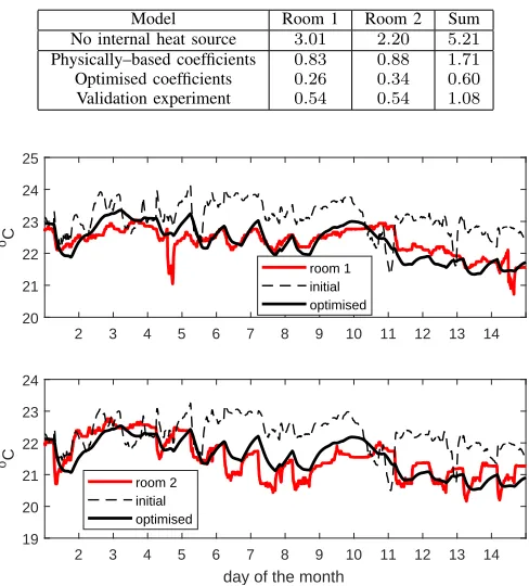
coefficients that further reduce the modelling errors. While most parameters remain close to the calculated values, the estimated resistance between the rooms is increased by a factor of ten. Further research is required into this and related optimisation issues but, in this particular example, higher resistances might be explained by the fact that storage units are placed along the wall on both sides of the glass partition. The middle rows of Table V compare the MAE for the initial (based on the values in Table IV) and optimised coefficients, while Fig. 4 shows the time responses. The MAE values are much reduced but Fig. 4 shows that there remains scope for further improvement in the model fit, and additional research is also required into model identifiability. Nonetheless, these preliminary results suggest that numerical optimisation of the parameters from BMS data, using initial conditions based on the physically determined values, is a viable approach.
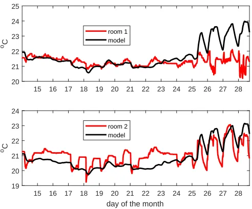
Finally, Fig. 5 and the bottom row of Table V show the results from a typical validation experiment, in which the
TABLE V
SUM OF MEAN ABSOLUTE ERROR BETWEEN DATA AND MODEL RESPONSE.
Model Room 1 Room 2 Sum
No internal heat source 3.01 2.20 5.21 Physically–based coefficients 0.83 0.88 1.71 Optimised coefficients 0.26 0.34 0.60 Validation experiment 0.54 0.54 1.08
2 3 4 5 6 7 8 9 10 11 12 13 14 20
21 22 23 24 25
oC
room 1 initial optimised
2 3 4 5 6 7 8 9 10 11 12 13 14 day of the month
19 20 21 22 23 24
oC
room 2 initial optimised
Fig. 4. Model estimation: measured room temperatures (red) for the first two weeks of September 2017, compared with the output of a model that includes an internal heat source. The response of an initial model with physically– based coefficients (dashed) is compared to the response with coefficients that have been numerically optimised to fit these data (solid).
thermal model is simulated using the input signals for the final two weeks of September 2017, whilst the coefficients are those estimated above. The magnitude of the room temperatures are broadly correctly predicted, especially for room one during the first 10 days. It is noteworthy, however, that the model overestimates the temperature in room one towards the end of the simulation experiment: this is associated with the change in HVAC activity for the last few days of September (see section III). In this regard, one option might be to develop a scheduled modelling approach, with different coefficients and settings for heating and air conditioning scenarios.
VI. ANALYSIS ANDDISCUSSION
Denoting s =d/dt, equations (3) and (4) yields Transfer Function models for room temperature. Introducing the heat input (6), substituting forqi and grouping parameters yields,
T1= b1 A1(s)
Ts1+ b2 A1(s)
TE+
b3 A1(s)
T2+ b4 A1(s)
U1 (7)
T2= b5 A2(s)
Ts2+ b6 A2(s)
TE+
b7 A2(s)
T1+ b8 A2(s)
U2 (8)
where,
A1(s) =C1R1R12s+ ˙m1cpR1R12+R1+R12
15 16 17 18 19 20 21 22 23 24 25 26 27 28 20
21 22 23 24 25
oC
room 1 model
15 16 17 18 19 20 21 22 23 24 25 26 27 28 day of the month
19 20 21 22 23 24
oC
[image:5.612.51.297.47.251.2]room 2 model
Fig. 5. Model validation: measured room temperatures (red) for the final two weeks of September 2017, compared with the output of a model that includes an internal heat source (and which has been numerically optimised for data collected during thefirsttwo weeks of September).
b1= ˙m1cpR1R12 ; b2=R12 ; b3=R1 ; b4=R1R12
b5= ˙m2cpR2R12 ; b6=R12 ; b7=R2 ; b8=R2R12
In principle the composite parameters stated above can be estimated from the BMS data using techniques from the system identification literature e.g. the RIV algorithm in the CAPTAIN toolbox [18]. Furthermore, generalising this formulation by defining e.g.A(s) =sn+. . .+an−1s+an, in
whichnis the polynomial order, allows for the identification of higher order model structures that are not necessarily limited to the 1R1C form assumed above. However, since the room temperatures are dependent on each other, multi–input, single– output (MISO) estimation using the standard RIV algorithm may yield biased estimates of the parameters, and this is the subject of current research by the authors.
Consideration of a first order Transfer FunctionK/(τ s+1), where τ is the time constant andK is the steady state gain, yields the following time constants for the thermal model,
TC(T1) =
C1R1R12
˙
m1cpR1R12+R1+R12
(9)
TC(T2) =
C2R2R12
˙
m2cpR2R12+R2+R12
(10)
Furthermore, the component steady state gains are obtained by settings= 1 in each Transfer Function model. Hence, for illustration, assuming time–invariantTs,1,TEandT2, together
with U1 =U2= 0 (i.e. the initial model without an internal
heat source), yields,
T1(t→ ∞) =
˙
mfcpR1R12TS,1+R12TE+R1T2
˙
m1cpR1R12+R1+R12
(11)
In this case, using the physically–based parameters in Ta-ble IV, less than 0.03% of the output is associated with the supply temperature, with 81% from the external temperature
and19% from the second room temperature, hence the poor performance of this initial model is perhaps not too surpris-ing. Furthermore, because of the constrained nature of the composite parameters in the Transfer Function (and regardless of the numerical value of each physical coefficient), the sum of the component steady state gains equals unity – the room temperature is always the weighted (summed to unity) sum of each steady state input temperature. This is inconsistent with the Charles Carter Building September 2017 data, in which the room temperatures are a degree or two hotter than all the supply (and external) temperatures, and hence provides further motivation for the introduction of the internal heat source.
To improve on the time–invariant heat source introduced by equation (6), the model is further developed to address how the occupancy levels vary over the course of the day in different parts of the building. Two sets of data gathered by the BMS are combined: the number of devices connected to the Wi-Fi hubs and the returning CO2 levels. There are
four Wi-Fi hubs in the Charles Carter Building, one per floor, which log the total number of connected devices every 10 minutes. As the staff and research student offices have desktop PCs with a wired connection, one device per person seems a reasonable approximation, and proves to work well in practice. Furthermore, this approach is appealing since existing sensors and readily available data sets are used i.e. there is scope for general implementation throughout the university, without requiring the installation of bespoke sensors.
However, since there is only one Wi-Fi hub per floor, this count provides no insight into to how the occupants are distributed between different rooms or zones on the floor. The latter is provided by the relative changes in CO2 levels. To
illustrate the approach, A–floor is divided into five zones, each served by one Air Handling Unit (AHU), with the occupancy in the new model represented as follows,
An(t) =P(t) Hn(t+b)−min(Hn)
P5
n=1(Hn(t+b)−min(Hn))
(12)
whereAn(t)represents the number of occupants in zonenat
timet,Hn(t)the CO2 level (ppm) in zonenat timet,P(t)
is the total number of occupants on this floor as recorded by the Wi-Fi hub, andb is the time–delay.
For a preliminary evaluation, a head count or ‘ground truth’ measurement was taken by the first author every 10 minutes during a week day in September 2018 (Fig. 6). Unfortunately, since this date does not fall during term time, the building was relatively under-occupied. In particular, in the late morning both meeting rooms were fully occupied by attendees who may have switched off their devices, zones 11 and 12, whilst the rest of the floor was largely unoccupied. During busier days, the results would not be dominated by the meeting rooms in this way, although further research by the authors into such issues is on-going. However, even for this limited example, Fig. 6 suggests that the CO2and Wi-Fi data provide
Fig. 6. Estimated and observed (‘ground truth’) occupancy for four zones on floors B and C, for an illustrative day outside of term time, September 2018.
VII. CONCLUSIONS
A simplified model of two rooms in a building on Lancaster University’s campus has been developed using the thermal– electrical analogy. Using physically derived parameters yields unsatisfactory model performance but this is significantly improved when an internal heat source is added and the coef-ficients are numerically optimised using data from the BMS. Although the two–room model and equivalent transfer function form reported in the present article provide useful insight into the thermal–electrical concept, for representation of an entire building a state space formulation will be utilised [22].
On the university campus, an energy centre provides the hot water that is used to heat the buildings on the network, and contains multiple methods of heat production, such as gas boilers and a biomass generator. Therefore, in future research, this type of model will be used to explore options for a hierarchical control system, with a particular focus on optimising the use of the boilers and generator. In this regard, the authors are presently developing demand–side control concepts to address multiple buildings on this network i.e. the control actions for one building are accounted for when choosing actions for the other buildings. This will be achieved within a non-minimal state space model predictive control framework [23]–[25]. Moreover by incorporating weather into the control system and so making full use of the available data from the local Hazelrigg weather station, it is anticipated the entire network can be better optimised.
ACKNOWLEDGMENTS
This work is supported by the UK Engineering and Physical Sciences Research Council (EPSRC) grant EP/M015637/1.
REFERENCES
[1] L. Price, P. C. Young, D. Berckmans, K. Janssens, and C. J. Taylor, “Data–based mechanistic modelling (DBM) and control of mass and energy transfer in agricultural buildings,”Annual Reviews in Control, vol. 23, pp. 71–83, 1999.
[2] O. Tate, E. D. Wilson, D. Cheneler, and C. J. Taylor, “Computational fluid dynamics and data–based mechanistic modelling of a forced ventilation chamber,” in18th IFAC Symposium on System Identification (SYSID), Stockholm, Sweden, July 2018.
[3] R. Yang and L. Wang, “Multi–zone building energy management using intelligent control and optimization,” Sustainable Cities and Society, vol. 6, no. 1, pp. 16–21, 2013.
[4] S. H. Kim, “Building demand–side control using thermal energy storage under uncertainty: An adaptive multiple model–based predictive control (MMPC) approach,”Building and Environment, vol. 67, pp. 111–128, 2013.
[5] S. Goyal, H. A. Ingley, and P. Barooah, “Occupancy–based zone–climate control for energy–efficient buildings: Complexity vs. performance,”
Applied Energy, vol. 106, pp. 209–221, 2013.
[6] B. Kossak and M. Stadler, “Adaptive thermal zone modeling including the storage mass of the building zone,”Energy and Buildings, vol. 109, pp. 407–417, 2015.
[7] B. Mayer, M. Killian, and M. Kozek, “Hierarchical model predictive control for sustainable building automation,”Sustainability, vol. 9, no. 264, pp. 1–20, 2017.
[8] A. Foucquier, S. Robert, F. Suard, L. St´ephan, and A. Jay, “State of the art in building modelling and energy performances prediction: A review,”Renewable and Sustainable Energy Reviews, vol. 23, pp. 272– 288, 2013.
[9] V. Paschkis and H. D. Baker, “A method for determining unsteady-state heat transfer by means of an electrical analogy,”Transactions ASME, vol. 64, pp. 105–112, 1942.
[10] E. Ramirez-Laboreo, C. Sagues, and S. Llorente, “Thermal modeling, analysis and control using an electrical analogy,” in22nd Mediterranean Conference on Control and Automation, Palermo, Italy, 2014. [11] C. Peng and Z. Wu, “Thermoelectricity analogy method for computing
the periodic heat transfer in external building envelopes,” Applied Energy, vol. 85, no. 8, pp. 735–754, 2008.
[12] Q. Chen, R.-H. Fu, and Y.-C. Xu, “Electrical circuit analogy for heat transfer analysis and optimization in heat exchanger networks,”Applied Energy, vol. 139, pp. 81–92, 2015.
[13] G. Fraisse, C. Viardot, O. Lafabrie, and G. Achard, “Development of a simplified and accurate building model based on electrical analogy,”
Energy and Buildings, vol. 34, no. 10, pp. 1017–1031, 2002. [14] J. M. Penman, “Second order system identification in the thermal
response of a working school,”Building and Environment, vol. 25, no. 2, pp. 105–110, 1990.
[15] M. M. Gouda, S. Danaher, and C. P. Underwood, “Building thermal model reduction using nonlinear constrained optimization,”Building and Environment, vol. 37, no. 12, pp. 1255–1265, 2002.
[16] S. Goyal and P. Barooah, “A method for model-reduction of non-linear thermal dynamics of multi-zone buildings,”Energy and Buildings, vol. 47, pp. 332–340, 2012.
[17] S. Klein, W. Beckman, and P. Cooper, TRNSYS: A Transient System Simulation Program. Solar Energy Laboratory, University of Wisconsin, Madison, Wisconsin, 1978.
[18] C. J. Taylor, P. C. Young, W. Tych, and E. D. Wilson, “New develop-ments in the CAPTAIN Toolbox for Matlab,” in18th IFAC Symposium on System Identification (SYSID), Stockholm, Sweden, July 2018. [19] V. Tabak and B. de Vries, “Methods for the prediction of intermediate
activities by office occupants,”Building and Environment, vol. 45, no. 6, pp. 1366–1372, 2010.
[20] Z. Yang and B. Becerik-Gerber, “Modeling personalized occupancy profiles for representing long term patterns by using ambient context,”
Building and Environment, vol. 78, pp. 23–35, 2014.
[21] M. Luo, Z. Wang, K. Ke, B. Cao, Y. Zhai, and X. Zhou, “Human metabolic rate and thermal comfort in buildings: The problem and challenge,”Building and Environment, vol. 131, pp. 44–52, 2018. [22] O. Tate, D. Cheneler, and C. J. Taylor, “A thermal–electrical analogy
model of a four–floor building with occupancy estimation for heating system control,” in 5th IFAC Conference on Intelligent Control and Automation Sciences (ICONS), Belfast, UK, August 2019.
[23] L. Wang, P. C. Young, P. J. Gawthrop, and C. J. Taylor, “Non–minimal state–space model–based continuous–time model predictive control with constraints,”International Journal of Control, vol. 82, no. 6, pp. 1122– 1137, 2009.
[24] V. Exadaktylos and C. J. Taylor, “Multi–objective performance optimi-sation for model predictive control by goal attainment,”International Journal of Control, vol. 83, no. 7, pp. 1374–1386, 2010.