Galaxies in X ray Selected Clusters and Groups in Dark Energy Survey Data II: Hierarchical Bayesian Modeling of the Red Sequence Galaxy Luminosity Function

MNRAS000,1–16(2019) Preprint 2 July 2019 Compiled using MNRAS LA_{TEX style file v3.0}

Galaxies in X-ray Selected Clusters and Groups in Dark Energy

Survey Data II: Hierarchical Bayesian Modeling of the

Red-Sequence Galaxy Luminosity Function

Y. Zhang

, C. J. Miller

, P. Rooney

, A. Bermeo

, A. K. Romer

, C. Vergara Cervantes

,

E. S. Ryko

ff

, C. Hennig

, R. Das

, T. McKay

, J. Song

, H. Wilcox

, D. Bacon

, S. L. Bridle

,

C. Collins

, C. Conselice

, M. Hilton

, B. Hoyle

, S. Kay

, A. R. Liddle

, R. G. Mann

,

N. Mehrtens

, J. Mayers

, R. C. Nichol

, M. Sahlén

, J. Stott

, P. T. P. Viana

, R. H. Wechsler

,

T. Abbott

, F. B. Abdalla

, S. Allam

, A. Benoit-Lévy

, D. Brooks

, E. Buckley-Geer

,

D. L. Burke

, A. Carnero Rosell

, M. Carrasco Kind

, J. Carretero

, F. J. Castander

,

M. Crocce

, C. E. Cunha

, C. B. D’Andrea

, L. N. da Costa

, H. T. Diehl

, J. P. Dietrich

,

T. F. Eifler

, B. Flaugher

, P. Fosalba

, J. García-Bellido

, E. Gaztanaga

, D. W. Gerdes

,

D. Gruen

, R. A. Gruendl

, J. Gschwend

, G. Gutierrez

, K. Honscheid

, D. J. James

,

T. Jeltema

, K. Kuehn

, N. Kuropatkin

, M. Lima

, H. Lin

, M. A. G. Maia

, M. March

,

J. L. Marshall

, P. Melchior

, F. Menanteau

, R. Miquel

, R. L. C. Ogando

, A. A. Plazas

,

E. Sanchez

, M. Schubnell

, I. Sevilla-Noarbe

, M. Smith

, M. Soares-Santos

, F. Sobreira

,

E. Suchyta

, M. E. C. Swanson

, G. Tarle

, A. R. Walker

(DES Collaboration)

Author affiliations are listed at the end of this paper.

Accepted XXX. Received YYY; in original form ZZZ

ABSTRACT

Using ∼100 X-ray selected clusters in the Dark Energy Survey Science Verification data,

we constrain the luminosity function (LF) of cluster red sequence galaxies as a function of redshift. This is the first homogeneous optical/X-ray sample large enough to constrain the evolution of the luminosity function simultaneously in redshift (0.1<z<1.05) and cluster mass (13.5≤log10(M200crit)∼<15.0). We pay particular attention to completeness issues and the detection limit of the galaxy sample. We then apply a hierarchical Bayesian model to fit the cluster galaxy LFs via a Schecter function, including its characteristic break (m∗) to

a faint end power-law slope (α). Our method enables us to avoid known issues in similar

analyses based on stacking or binning the clusters. We find weak and statistically insignificant (∼1.9σ) evolution in the faint end slopeαversus redshift. We also find no dependence inα orm∗with the X-ray inferred cluster masses. However, the amplitude of the LF as a function

of cluster mass is constrained to ∼20% precision. As a by-product of our algorithm, we

utilize the correlation between the LF and cluster mass to provide an improved estimate of the individual cluster masses as well as the scatter in true mass given the X-ray inferred masses. This technique can be applied to a larger sample of X-ray or optically selected clusters from the Dark Energy Survey, significantly improving the sensitivity of the analysis.

Key words:galaxies: evolution - galaxies: clusters: general

? _{Yuanyuan Zhang:[email protected]}

1 INTRODUCTION

Galaxy clusters are special for both cosmology and astrophysics studies. As the structures that correspond to the massive end of halo mass function, they are sensitive probes of theΛCDM

mological model (see reviews inAllen et al. 2011;Weinberg et al. 2013). As the most massive virialized structures in the universe, they provide the sites for studying astrophysical processes in dense environments.

Galaxy clusters are known to harbor red sequence (RS) galax-ies, so named because these galaxies rest on a tight relation in the color-magnitude space (Bower et al. 1992). The phenomenon has been employed in finding clusters from optical data (e.g.,Gladders & Yee 2000;Miller et al. 2005;Koester et al. 2007;Rykoffet al. 2016;Oguri et al. 2018) and developing cluster mass proxies (e.g.,

Rykoffet al. 2012). Red sequence galaxies also attract attention in astrophysics studies as they exhibit little star formation activity. Their formation and evolution provide clues to how quenching of galaxy star formation occurs in the cluster environment.

It is well-established that the massive red sequence galaxies form at an early epoch (e.g., Mullis et al. 2005; Stanford et al. 2005;Mei et al. 2006;Eisenhardt et al. 2008;Kurk et al. 2009;

Hilton et al. 2009;Papovich et al. 2010;Gobat et al. 2011;Jaffé et al. 2011;Grützbauch et al. 2012;Tanaka et al. 2013), but the formation of faint red sequence galaxies can be better character-ized. The latter could be examined through inspecting the luminos-ity distribution of cluster galaxies, either with the dwarf-to-giant ratio approach (De Lucia et al. 2007), or as adopted in this paper, with a luminosity function (LF) analysis. Results from these anal-yses are controversial to date, and have been extensively reviewed in literature (e.g.,Faber et al. 2007;Crawford et al. 2009;Boselli & Gavazzi 2014;Wen & Han 2015).

To summarize, a few studies have reported a deficit of faint red sequence galaxies with increasing redshift (De Lucia et al. 2007;

Stott et al. 2007;Gilbank et al. 2008;Rudnick et al. 2009;Capozzi et al. 2010;de Filippis et al. 2011;Martinet et al. 2015;Lin et al. 2017), indicating later formation of faint red sequence galaxies compared to the bright (and massive) ones. Yet, many other works observe little evolution in the red sequence luminosity distribution up to redshift 1.5 (Andreon 2008;Crawford et al. 2009;De Pro-pris et al. 2013,2015,2016;Cerulo et al. 2016;Connor et al. 2017;

Sarron et al. 2018), suggesting an early formation of both faint and bright red sequence galaxies. Differences in these results are hard to interpret given the different methods (see the discussion in Craw-ford et al. 2009), sample selections and possible dependence on cluster mass (Gilbank et al. 2008;Hansen et al. 2009;Lan et al. 2016), dynamical states (Wen & Han 2015;De Propris et al. 2013), and whether or not the clusters are fossils (Zarattini et al. 2015). Carrying out more detailed analyses, especially in the 0.5 to 1.0 redshift range, may help resolve the differences.

The luminosity distribution of cluster galaxies has also been modeled to connect galaxies with the underlying dark matter distri-bution. The luminosity function of galaxies in a halo/cluster of fixed mass, entitled the conditional luminosity function (CLF) in the lit-erature (Yang et al. 2003), statistically models how galaxies oc-cupy dark matter halos. Modeling the Halo Occupation Distribution (HOD,Peacock & Smith 2000;Berlind & Weinberg 2002;Bullock et al. 2002) provides another popular yet closely-related approach. Given a dark matter halo distribution, these models (HOD & CLF) can be linked with several galaxy distribution and evolution prop-erties (e.g.,Popesso et al. 2005;Cooray 2006;Popesso et al. 2007;

Zheng et al. 2007;van den Bosch et al. 2007;Zehavi et al. 2011;

Leauthaud et al. 2012;Reddick et al. 2013), including galaxy cor-relation functions (e.g.,Jing et al. 1998;Peacock & Smith 2000;

Seljak 2000), galaxy luminosity/stellar mass functions (e.g.,Yang et al. 2009), global star formation rate (e.g.,Behroozi et al. 2013) and galaxy-galaxy lensing signals (e.g.,Mandelbaum et al. 2006).

Furthermore, LF & HOD analyses improve our understanding of the cluster galaxy population. The number of cluster galaxies, especially the number of cluster red sequence galaxies, is a useful mass proxy for cluster abundance cosmology. Deep optical surveys like the Dark Energy Survey (DES1_{,DES Collaboration 2005)}

de-mand refined understanding of the evolution of cluster galaxies to

z=1.0 (Melchior et al. 2017) .

The Sloan Digital Sky Survey (SDSS2) has enabled detailed analysis of the cluster LFs (or CLFs) with the identification of tens of thousands of clusters to redshift 0.5 (Yang et al. 2008;Hansen et al. 2009). Above redshift 0.5, most studies have been performed with relatively small samples containing a handful of clusters or groups (Andreon 2008;Rudnick et al. 2009;Crawford et al. 2009;

De Propris et al. 2013;Martinet et al. 2015;De Propris 2017) and wide field surveys that are more sensitive than SDSS have just pro-vided an opportunity to reinvigorate such analyses (Sarron et al. 2018).

In this paper, we constrain the (conditional) red sequence lu-minosity function (RSLF) with an X-ray selected cluster sample (details in Section2.3) detected in the DES Science Verification (DES-SV) data including the supernovae data sets collected during the same time. Clusters selected with the same approach are used in a cluster central galaxy study inZhang et al.(2016), but with an updated X-ray archival data set. The sample contains∼100 clusters and groups in the mass range of 3×1013 Mto 2×1015 M, and the redshift range of 0.1 to 1.05. To date, it still represents a cluster sample that is complete to the highest redshift range discovered in DES, owing to the full depth data sets collected during DES-SV. As the clusters are not selected by their red sequence properties, study-ing RSLF with the sample is not subject to red sequence selection biases. Similar analyses can also be applied to SZ-selected clusters (e.g., clusters discovered from the South Pole Telescope survey:

Bleem et al. 2015;Hennig et al. 2017) and clusters selected from optical data. Our paper focuses on cluster red members. The lumi-nosity function of blue galaxies generally deviates from that of the red, but the red cluster members are easier to select photometrically due to the tightness of the color-magnitude relation.

The number of member galaxies in low mass clusters is often too low to study LFs for individual systems. It is a common ap-proach to stack the member galaxy luminosity distributions for an ensemble of clusters (e.g., Yang et al. 2009;Hansen et al. 2009). In this paper, we develop a hierarchical Bayesian modeling tech-nique. The method allows us to acquire similar results to a stacking method, with the added benefits of robust uncertainty estimation and simultaneous quantification of the possible mass dependence and redshift evolution effects. In the rest of the paper, we first in-troduce our data sets in Section2and then describe the methods in Section3. The results are presented in Section4. Discussions of the methods and results as well as a summary of the paper are presented in Section5.

2 DATA

2.1 Dark Energy Survey Science Verification Data

We use the DES Science Verification (DES-SV) data taken in late 2012 and early 2013. The DES collaboration collected this data set with the newly mounted Dark Energy Camera (DECam, Flaugher

et al. 2015) for science verification purposes before the main survey began (for details on DES Year 1 operations, seeDiehl et al. 2014). In total, the data set covers∼400 deg2of the sky. For about 200 deg2, data are available3in all of theg,r,i,zandYbands, and the total exposure time in each band fulfills DES full depth requirement (23 to 24 mag iniand 22 to 23 mag inz, see more details inSánchez et al. 2014). A pilot supernovae survey (see Papadopoulos et al. 2015, for an overview) of 30 deg2sky ing,r,i,zwas conducted at the same time, reaching deeper depth after image coaddition (∼25 mag iniand∼24 mag inz).

The DES-SV data are processed with the official DES data reduction pipeline (Sevilla et al. 2011;Mohr et al. 2012). In this pipeline, single exposure images are assessed, detrended, calibrated and coadded. The coadded images are then fed to the SExtractor software (Bertin & Arnouts 1996;Bertin 2011) for object detection and photometry measurement.

2.2 The DES Photometric Data

We use a DES value-added catalog, the “gold” data set (see the review inRykoffet al. 2016;Drlica-Wagner et al. 2018)4, based on catalogs produced from the SExtractor software. The detection threshold is set at 1.5σ(DETECT_THRESH = 1.5) with the default SExtractor convolution filter. The minimum detection area is set at 6 pixels5 (DETECT_MINAREA =6). The SExtractor runs were per-formed in dual mode, using the linear addition ofr,iandzband images as the detection image.

The “gold” data set is subsequently derived with the initial de-tections, keeping only regions that are available in all of theg,r,i,

zbands. Regions with a high density of outlier colors due to the im-pact of scattered light, satellite or airplane trails, and regions with low density of galaxies near the edge of the survey are removed. Objects near bright stars selected from the Two Micron All Sky Survey (2MASSSkrutskie et al. 2006) are masked. The masking radius scales with stellar brightness inJasRmask=150−10J

(arc-seconds) with a maximum of 120 arcseconds (Jarvis et al. 2016;

Rykoffet al. 2016). Stars of nominal masking radii less than 30 arcseconds are not masked to avoid excessive masking. Coverage of the sample is recorded with the HEALPix6 software (Górski et al. 2005) gridded byN=4096. Photometry are re-calibrated and extinction-corrected using the Stellar Locus Regression technique (SLR:Kelly et al. 2014).

We make use of the SExtractor Kron magnitudes (mag_auto,

Kron 1980) for all detected objects. Since the SExtractor run was performed in dual mode, the Kron aperture and the centroid for different filters are the same, which are determined from the de-tection images. The luminosity functions are derived with DES

z−band photometry, based on objects>5σ(which corresponds to magerr_auto_z<2.5/ln10/5=0.218mag).

We derive completeness limits for the selected>5σobjects. Details of the completeness analyses are provided in AppendixA. In general, the completeness limits are∼0.5mag brighter than the sample’s 10σ depth magnitudes. The selected >5σ objects are >99.8% complete above the limits. Because of this high complete-ness level, we do not correct for incompletecomplete-ness in this paper.

3 _{http://des.ncsa.illinois.edu/releases/sva1} 4 _{https://des.ncsa.illinois.edu/releases/sva1} 5 _{DECam pixel scale 0.263”}

6 _{http://healpix.sourceforge.net}

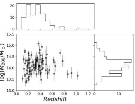
Figure 1.The XCS-SV clusters: redshifts, masses, and mass uncertainties. The upper and right histograms respectively show the cluster redshift and mass distribution.

2.3 The XCS-SV cluster sample

The XCS-SV cluster sample is a product from theXMMCluster Survey (Lloyd-Davies et al. 2011;Mehrtens et al. 2012;Viana et al. 2013), which searches for galaxy cluster candidates (extended X-ray emissions) in theXMM-Newtonarchival data. The X-ray se-lected cluster candidates (about 300 in number) are later confirmed with the DES-SV optical images, and have their photometric red-shifts estimated using the DES-SV photometric data set. The XCS-SV sample contains galaxy groups, low mass clusters and clusters as massive as 1015Mto beyond redshift 1. Selection and confirma-tion methods of the sample, as well as the cluster photometric red-shift measurements are reviewed inZhang et al.(2016, henceforth referenced as Z16). The sample used in this paper are expanded from that in Z16 after finalizing the input X-ray data. We make use of only the clusters of which the mass uncertainties, derived from the X-ray temperature measurements, are less than 0.4 dex.

Since this paper evaluates luminosity function with thez-band photometry, we eliminate clusters above redshift 1.05 for which the rest-frame 4000Å break of RS galaxies have shifted out of DESz−band coverage (sensitive to∼8500 Å). We only use clus-ters located in DES-SV regions with the analysis magnitude ranges (above characteristic magnitude+2 mag) above the completeness limits (Section 2.2). The paper works with 93 clusters in total, which are listed in AppendexB, TableB. In Figure1, we show the redshifts, masses, and mass uncertainties of the analyzed clusters.

The cluster masses and uncertainties are derived from X-ray temperature based on a literatureTX−M relation (Kettula et al.

2013) (see details also in Z16).R200is derived fromM200.

2.4 Red Sequence Galaxy Selection

The definition of cluster member galaxies in projected datasets is a difficult challenge. Our method is based on simple color cuts around the cluster red sequence (De Lucia et al. 2007;Stott et al. 2007;Gilbank et al. 2008;Crawford et al. 2009;Martinet et al. 2015). To account for the shifting of the 4000 Å break, we select red sequence galaxies according tog−r color atz<0.375,r−i

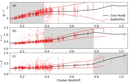
Figure 2.Observer-frameg−r(panel a),r−i(panel b) andi−z(panel c) colors of the cluster red sequence candidates (red data points) and the red sequence model (black solid lines). Note that the color distributions of cluster foreground/background objects are not subtracted. We also show the 2σcolor ranges of red sequence cluster members (member probability> 50% ) from the redMaPPer DES-SV cluster sample (Rykoffet al. 2016) for comparison, which appear to agree with our color models.

For a cluster at redshiftz, we first apply K-corrections ( Blan-ton & Roweis 2007) to all the objects in the cluster field. These objects are band-shifted to a reference redshift (depending on the color choice), assuming the cluster redshift to be their original red-shifts. We compare the corrected colors to a model color with the following standard:

|(g−r)z=0.25−(g−r)model atz=0.25|<

q δ2

g−r+ ∆2g−r,or

|(r−i)z₌0.55−(r−i)model atz=0.55|<

q δ2

r−i+ ∆

2

r−i,or

|(i−z)z=0.9−(r−i)model atz=0.9|<

q δ2

i−z+ ∆

2

i−z.

(1)

In these equations, the model colors (g−r, r−i, ori−z, details explained below) are the mid-points of a selection window at a ref-erence redshift.δg−r,δr−iandδi−zare the photometry uncertainties. ∆g−r,∆r−iand∆i−zare the widths of the selection windows.

We set∆g−r to be 0.2 mag. The clipping width is chosen to be larger than the combination of the intrinsic scatter and the slope of red sequence color-magnitude relations, while avoiding a signif-icant amount of blue galaxies.∆r−iis adjusted to be 0.15 through matching the number of selected cluster galaxies (after background subtraction, see Section3.2for details) to fiducialg−rselections at 0.3≤z<0.5.∆i−zis adjusted to be 0.12 through matching the number of selected cluster galaxies (after background subtraction, see Section3.2for details) to fiducialr−iselections atz≥0.7.

The model colors ofg−ratz=0.25,r−iatz=0.55 and i−zatz=0.9 are based on a simple stellar population template

from Bruzual & Charlot(2003), assuming a single star burst of metallicityZ=0.008 atz=3.0, computed with the EZGal

pack-age7(Mancone & Gonzalez 2012). In Figure2, we show the red sequence model, over-plotting the observer frame colors of the se-lected objects. Overall, the colors of the sese-lected RS candidates match template well. The template also matches the colors of clus-ter red sequence defined by the RedMaPPer method (Rykoffet al. 2016).

7 _{http://www.baryons.org/ezgal/}

For RS candidates selected with the above criteria, we em-ploy a statistical background subtraction approach (see details in Section3) to eliminate background objects, which on average con-stitute 50% of the cluster region galaxies brighter thanm∗+2 mag. The performance of star-galaxy classifiers applied to the DES SVA1 “gold" sample (Section2.2) depends on the object’s apparent magnitude. The classifiers become unstable for objects fainter than ∼22 mag in thez−band. Since it is possible to eliminate the stellar contamination with the background subtraction procedure (we esti-mate the background object –stellar and galactic– densities locally for each cluster), we do not attempt to separate stars and galaxies among the RS candidates (above 21 mag inz, stars make up∼10% of the sample). We nevertheless refer to all objects as “galaxies”.

3 METHODS

The main results in this paper are derived with a hierarchical Bayesian method (application examples to cosmology can be found in Loredo & Hendry 2010). We constrain the RSLF with a sin-gle Schechter function (Schechter 1976) to the magnitude limit of

m∗+2 mag, and simultaneously model the mass and redshift de-pendence of the parameters (Section3.1: a hierarchical Bayesian method). To test the method, we compare the constraints to results derived from stacking cluster galaxy number counts in luminosity bins (Section3.2: alternative histogram method).

Generally, the input to both methods includes the observed magnitudes,{mi}, of objects inside clusters or in a "field" region (miis the apparent magnitude of theith object). We define the clus-ter region as enclosed within 0.6R200of the cluster centers (X-ray

centers). The contrast between cluster and background object den-sities is large with this choice (excess cluster object density to back-ground object density about 1:1 for most of the clusters throughout the DES-SV depth), and the amount of retained cluster galaxies is reasonable. We choose the field region to be annular, centered on the cluster, with the inner and outer radii being 3R200and 8R200

re-spectively. The choice helps eliminating RSLF contributions from cluster-correlated large scale structures along the line-of-sight. The cluster central galaxies selected according to the criteria in Z16 are eliminated from the analysis. Central galaxies are known to be out-liers to a Schechter function distribution. Their properties and halo occupation statistics are investigated in Z16.

The area of these regions are traced with randomly generated locations that have uniform surface density across the “gold" sam-ple footprint, i.e., a samsam-ple of “random points”. For each cluster, we generate∼1.5 million random points within 10R200. The number

density is high enough that the resulting uncertainty is negligible (∼1% in the luminosity distribution measurements). We ignore the uncertainties from using random points.

3.1 A Hierarchical Bayesian Method

Given a model with a set of parametersΩthat describes the dis-tribution of observables, Bayesian theory provides a framework for inferringΩwith a set of observed quantities{x}. In this sub-section, we describe the methods developed in this framework.

Denoting the probability of observing{x}in modelΩto be

P({x}|Ω), and the prior knowledge about the model parameters to beP(Ω), after observations of{x}, the Bayes’ theorem updates the knowledge about model parameters, namely the posterior distribu-tion, to be:

The above equation uses a proportional sign instead of an equal sign as a probability function needs to be normalized to 1. The nor-malization factor is un-interesting when the posterior probability is sampled with Markov Chain Monte Carlo.

In our application, the observables include the observed mag-nitudes of objects in the cluster or field region. A major compo-nent of our model is the Schechter function. The parameters of the Schechter function vary for clusters of different masses and red-shifts. Our model, called thehierarchicalmodel, assumes redshift and mass dependences for the faint end slope and the characteris-tic magnitude. For the parameter priorsP(Ω), we assume them to be flat for most of the parameters excluding a couple. The prior distributions are noted later when we introduce the parameters.

3.1.1 Basic Components of the Model

Forone cluster galaxy, we assume that the probability of observ-ing it with magnitudemfollows a Schechter function:

f(x)=ψf(0.4ln10)100.4(m

∗_−x)(α+1)

exp(−100.4(m∗−x)) (3) In this equation,ψf is the normalization parameter that normalizes

f(x) to 1.αandm∗are the faint end slope and the characteristic magnitude, treated as free parameters of the model.

For one object in thecluster region, it can be either acluster galaxyor afield object. For afield object, we denote the probability of observing it with magnitudemto beg(m).g(m) is approximated with a normalized histogram of the object magnitude distribution in the field region.

The probability of observing one object in the cluster region is the combination of observing it as afieldobjectandobserving it as aclustergalaxy. The probability writes

h(m)=ψh[Nclf(m)+Nbgg(m)] (4)

In this equation,Nclis the number of cluster galaxies in the cluster

region, andNbgis the number of field galaxies in the cluster region.

Again, there exists a normalization factorψh that normalizes the probability function to 1.

We treat the sum ofNbgandNclas a Poisson distribution. The

expected value ofNbgcan be extrapolated from the field region and

the area ratio between the cluster and the field regions. Equation4

introducesonefree parameter,Ncl, which controls the relative

den-sity between cluster and field galaxies in the cluster region.Nclcan

be further related to the amplitude of the Schechter function,φ∗ (in unit of total galaxy count), as the integration of the Schechter function over the interested magnitude range, written as

Ncl=

Z φ∗_f(m) ψf

dm

=_ψfφ∗

Z

f(m)dm.

(5)

Thus far, the free parameters in our models areα,m∗ from Equation3andφ∗. Note that, in this section, we only perform anal-yses with galaxies brighter than the completeness magnitude limit (galaxies are considered to be more than 99.8% complete through-out the analyzed magnitude range, according to SectionA).

We constrainφ∗with the number count of observed objects in the cluster region (N), assuming a Poisson distribution:

N∼ Poisson(Ncl+Nbg). (6)

The log-likelihood is explicitly written as:

logP(N)∝Nlog(Ncl+Nbg)−(Ncl+Nbg). (7)

For one cluster, we take the observables to be the observed magnitudes of cluster region objects,{mi}, the object number count andNand the background object number count.Nbgis treated as

a known quantity. The log-likelihood of observing these quantities is:

logP({mi},N|α,m∗,φ∗) ∝logP(N|φ∗,α,m∗)+X

i

logP({mi}|α,m∗,φ∗) ∝logP(N)+X

i

logh(mi).

(8)

3.1.2 Hierarchical Model

The Bayesian approach makes it possible to add dependences toα andm∗. We rewriteαandm∗with redshift or mass dependences:

αj=Aαlog(1+zj)+Bα(logMmodel,j−14)+Cα

m∗_z=0.4,j=Bm(logMmodel,j−14)+Cm.

(9) Here, we distinguish between true and observedM200of clusters.

logMmodel,jrepresents the trueM200mass of thejth cluster, while

we use logMobs,jto represent the M200mass derived from X-ray

temperature for thejth cluster. logMmodel,jfor different clusters are treated as free parameters in the analysis, but we use observational constraints on logM200 from X-ray data as priors (Gaussian

dis-tributions): logMmodel,j ∼ N(logMobs,j,σ2_M).σMis the

measure-ment uncertainty (including the intrinsic scatter and statistical un-certainties) of logMobs,jfrom X-ray data. The assumption about

logMmodel,j allows us to incorporate mass uncertainties into the

analysis. Furthermore, we constrainm∗ atz=0.4 (the mean and

median redshifts of the sample are 0.33 and 0.35 respectively) to be consistent with the redshift cut in the alternative method in Sec-tion3.2. For each cluster, we extrapolate them∗at its observedz

fromz=0.4 assuming a simple stellar population fromBruzual & Charlot(2003) with a single star burst of metallicityZ=0.008 at z=3.0 (the red sequence galaxy template used in Section2.4).

φ∗ _{for each cluster is constrained separately. We assume a} Gaussian prior distribution of{logφ∗_j}given the values predicted by the relation:φ∗_j∼ N(logφ∗

mean,j,σ

2

logφ).σlogφis the intrinsic scatter

of the relation, fixed at 0.58_{to reduce the number of free}

parame-ters. We further assume a power law relation betweenMmodel,jand φ∗

mean,j:

logφ∗

mean,j=Bφ×logMmodel,j+Cφ. (10)

The log likelihood of havingφ∗_jgivenMmodel,jwrites:

gj(φ∗_j)∝ − φ∗

j−(Bφ×logMmodel,j+Cφ)2

2σ2

logφ

(11)

The free parameters of this model areAα,Bα,Cα,Bm,Cm,Bφ,

Cφ,{φ∗

j}and{Mmodel,j}. The observed quantities are{mi,j}and{Nj}

of all clusters.{logMobs,j}are treated as priors for{logMmodel,j}. {zj}as well asNbg,jare treated as known quantities for each of the clusters. We summarize the model dependences with a schematic

8 _{Allowing the parameter to vary gives a scatter of∼0.2 to 0.3, and}

Figure 3.Schematic diagram of the hierarchical Bayesian method, as de-scribed in Section3.1. Note that Schechter function parameters likeαj,

m∗z=0.4,jandφ∗_j are not directly constrained in the model. Such

“parame-ters” (called pseudo parameters in the diagram), as well as known quantities are indicated by dashed line circles.

diagram in Figure3. The log-likelihood of observing these quanti-ties is:

logL({mi,j},{Nj}|Aα,Bα,Cα,Bm,Cm,Bφ,Cφ,{φ∗j},{Mmodel,j})

=logL({mi,j},{Nj}|αj,m∗j,{φ ∗

j})+logL({φ ∗

j}|{Mmodel,j})

∝X j

[logP(Nj|φ∗j,αj,m ∗ j)+

X

i

logP({mi,j}|αj,m∗j,φ ∗

j)]

+X j

logL(φ∗_j|Mmodel,j)

∝X j

[logPj(Nj)+X i

loghj(mi,j)+gj(φ∗_j)].

(12)

Finally, the parameter posterior likelihood is

logL(Aα,Bα,Cα,Bm,Cm,Bφ,Cφ,{φ∗_j},{Mmodel,j}|{mi,j},{Nj})

=logL({mi,j},{Nj}|αj,m∗_j,{φ∗_j})+logL({φ∗_j}|{Mmodel,j})

∝X j

[logP(Nj|φ∗j,αj,m ∗ j)+

X

i

logP({mi,j}|αj,m∗j,φ ∗

j)]

+X j

logL(φ∗_j|Mmodel,j)

+logL_prior(Aα,Bα,Cα,Bm,Cm,Bφ,Cφ,{φ∗_j},{Mmodel,j})

∝X

j

[logPj(Nj)+X i

loghj(mi,j)+gj(φ∗_j)]

+logL_prior(Aα,Bα,Cα,Bm,Cm,Bφ,Cφ,{φ∗_j},{Mmodel,j}).

(13)

We assume flat priors for most of the model parameters except

Cmandφj. ForCm, we assume a Gaussian distribution as the prior, with the measurement fromHansen et al.(2009) as the mean, and 1 mag2 as the variance. These priors are listed in Table1. Sam-pling from the parameter posterior likelihood is performed with the PyMC package (Fonnesbeck et al. 2015).

Figure 4.RSLFs derived in two redshift bins display a possible redshift evolution effect. Uncertainties with the data points are estimated through assuming Poisson distributions. The shaded bands show the fitted Schechter functions including 1σfitting uncertainties (with the method from Sec-tion3.2). Note that the data points have been rebinned from the input to the fitting method.

Figure 5.RSLFs derived in two cluster mass bins appear to be consistent. Uncertainties with the data points are estimated through assuming Poisson distributions. The shaded bands show the fitted Schechter functions includ-ing the 1σfitting uncertainties (with the method from Section3.2). Note that the data points have been rebinned from the input to the fitting method.

3.2 Alternative Histogram Method

We develop a separate method to test the fore-mentioned technique. This method starts with counting galaxies in magnitude bins. We use 150 bins from 15 mag to 30 mag spaced by 0.1mag. We do not see change of the results when adjusting the bin size from 0.2 mag to 0.05 mag.

The histogram counting is performed for the cluster region,

N(m), and the field region, N(m)background. To estimate the

con-tribution of field galaxies to the cluster histogram, we weight the number count of objects in the field region, with the random num-ber ratio:

Nbg(m)=N(m)background×

Nrandom,cluster

Nrandom,background

. (14)

Table 1.Prior and Posterior Distributions of the parameters (see Equa-tions9,10and10) in the Hierarchical Bayes Model

Prior Posterior

Aα [-5, 10] 1.30±0.70

Bα [-4, 4] −0.17±0.19

Cα [-2, 2] −0.77±0.16

Bm [-10, 10] −0.31±0.31

Cm N(−22.13,1.0) −22.19±0.19

atz=0.4 N(19.69,1.0) 19.63±0.19

Bφ [-5, 5] 0.73±0.13

Cφ [-10, 10] 0.85±0.08

cluster mass9, and also record the number count of clusters in each magnitude bin,C(m). During the summing process, we shiftmby the apparent magnitude difference beween the cluster redshift and a reference redshift (depending on the cluster redshift and mass binning) of a simple passively-evolving stellar population from

Bruzual & Charlot(2003) with a single star burst of metallicity

Z=0.008 atz=3.0 (the same red sequence galaxy template used in

Section2.4and 3.1.2). The histograms are then averaged for both the cluster region and the field region to obtain ¯N(m) and ¯Nbg(m).

Subtracting ¯Nbg(m) from ¯N(m) yields the luminosity distribution

of cluster galaxies (Figure4in redshift bins and Figure5in mass bins).

We assume a Schechter function distribution for cluster galax-ies:

S(m)=φ(0.4ln10)100.4(m∗−m)(α+1)exp(−100.4(m∗−m)), (15) therefore the expected number of galaxies in each magntiude bin in the cluster region is

E(m)=S(m)+Nbg(m). (16)

Assuming Poisson distributions for the number of galaxies in each bin, we sample from the following likelihood:

logL ∝X m

¯

N(m)C(m)log[E(m)C(m)]−E(m)C(m). (17) Sampling from the likelihood is performed with theemcee

package (Foreman-Mackey et al. 2013).

4 RESULTS

4.1 Results from Hierarchical Bayesian Modeling

The Hierarchical Bayes model (Section3.1.2) simultaneously con-strains the redshift evolution and mass dependence of αandm∗ anchored at redshift 0.4:

α=Aαlog(1+z)+Bα(logM200−14)+Cα

m∗_z=0.4=Bm(logM200−14)+Cm.

(18) Them∗at other redshifts are derived through evolving a pas-sive redshift evolution model described in Section3.1.2.

For each cluster, we only make use of the [m∗-2,m∗+2] magni-tude range. Galaxy members of the analyzed clusters are complete within this range by selection (see details in Section2.3). The con-straints of theαandm∗_z relations are listed in Table1. The model

9 _{Two clusters are further eliminated from the 93 cluster sample because}

they are severly masked and therefore do not reliably contribute to the stacked histograms.

Table 2.Fitted Schechter Function parameters in redshift/mass bins

Cluster Selection α m∗

0.1≤z<0.4 −0.80±0.12 18.17±0.18

64 clusters K-corrected toz=0.25

0.4≤z<1.05 −0.55±0.18 19.96±0.23

27 clusters K-corrected toz=0.49

13.2≤logM200<14.4 −0.67±0.12 19.48±0.17

77 clusters K-corrected toz=0.4

14.4≤logM200<15.1 −0.73±0.14 19.34±0.22

14 clusters K-corrected toz=0.4

posterior distributions are Gaussian-like according to visual checks. In Figure6, we plot theαandm∗zrelations as well as their uncer-tainties. For comparison, we show constraints from the alternative histogram approach (discussed in the following section).

The RSLF faint end slope,α, displays a weak evidence of red-shift evolution. TheAα parameter that controls the redshift evo-lution effect deviates from 0 at a significance level of 1.9σ. For clusters of logM200=14.1 (median mass of the cluster sample),α

is constrained to be−0.69±0.13 atz=0.2, rising to−0.52±0.14 at

z=0.6. The mass dependence ofαis ambiguous. TheBα parame-ter that controls this feature deviates from 0 by 0.9σ. The effect is likely degenerate with the mass dependence ofm∗. When removing

m∗mass dependence from the method (settingBmto be 0),Bαis consistent with 0.

We assume passive evolution to the RSLF characteristic mag-nitudem∗_z. We do not notice deviations ofm∗from the assumption (them∗ results in redshift and mass bins agree with the model). Although the method modelsm∗as mass-dependent, the effect ap-pears to be insignificant (Bmdeviates from 0 by 1.0σ).

The hierarchical Bayesian method also constrains the RSLF amplitudes,φ∗, and the relations betweenφ∗and logM200.φ∗scales

with the total number of cluster galaxies. Our result shows a strong correlation betweenφ∗and the cluster mass (Figure7).

4.2 Results in Redshift/Mass Bins

We divide the clusters into two redshift bins: 0.1≤z<0.4 and

0.4≤z<1.05 and apply the alternative histogram method

(Sec-tion 3.2)10. The median cluster masses in each of the bins are 1014.1M and 1014.16M respectively. The fitted parameters are listed in Table2. Results are also shown in Figure4and6. Again, the RSLF faint end slope,α, displays a hint of redshift evolution. The measurements in two redshift bins differ by∼1.2σ.

We divide the clusters into two mass bins: 13.2≤logM200<

14.4, 14.4≤logM200<15.1 and apply the alternative histogram

method. The median cluster redshifts in each of the bins are 0.35 and 0.34 respectively. To reduce uncertainties from band-shifting, we K-correct the RSLFs toz=0.4 (based on the red sequence

model in Section2.4). Results are presented in Table2, Figure5

and Figure6. No mass dependence of eitherαorm∗is noted. As shown in Figure6, the results in cluster redshift/mass bins agree with the extrapolations from the hierarchical Bayesian model (Section4.1) within 1σ.

10 _{The reshift/mass cuts of the histogram samples are chosen by judgement}

Figure 6. (Panels a and b) Redshift evolution of the faint end slope,α, and the characteristic magnitude,m∗(assuming passive redshift evolution of a simple stellar population from Bruzual & Charlot (2003) with a single star burst of metallicityZ=0.008 atz=3.0). (Panels c and d) Mass dependence of the faint end

slope,α, and the characteristic magnitude,m∗(assuming passive redshift evolution). Solid red lines and shades indicate results derived with the hierarchical Bayesian method (Section3.1). Solid red circles indicate results derived with the alternative histogram method (Section3.2). Literature reports of theαand

m∗parameters are over-plotted.

4.3 Comparison to Literature

In Figure6, we over-plot literature measurements of the RSLFα andm∗ parameters. In the comparison datasets,Andreon(2008),

Rudnick et al. (2009), Crawford et al.(2009),De Propris et al.

(2013), andMartinet et al. (2015) utilize smaller (Nclus =5-40) samples with individually measured LFs. For these, we compare to their stacked analyses when available since stacking reduce intrin-sic cluster-to-cluster variations, something we achieve naturally in our Bayesian hierarchical model. We note that our Bayesian anal-ysis utilizes a likelihood that is continuous in redshift, negating the need to stack our clusters in redshift bins (see Section3.1). We also include two low redshift constraints from stacked RSLFs on large cluster samples from the SDSS (Hansen et al. 2009;Lan et al. 2016). We do not compare to individual cluster RSLFs from the literature, since we do not have any known expectations on the cluster-to-cluster scatter in individual systems.

At low redshift, RSLF analyses based on SDSS data are avail-able from Hansen et al.(2009, z∼0.25) andLan et al. (2016,

z<0.05). The SDSS faint end slope measurements (Hansen et al. 2009) appear to be consistent with our results. The SDSS charac-teristic magnitudes appears to be slightly fainter than the values constrained in this paper, but still consistent within this paper’s 1σ uncertainties (Mz∗at redshift 0.4 is−22.0 from Lan et al. or−22.13 from Hansen et al., comparing to−22.19±0.19 in this paper). Note that the SDSS results are derived withr(Lan et al. 2016,z<0.05)

ori(Lan et al. 2016, z<0.05) band data and we assume a red

sequence model in Section2.4when comparing the characteristic magnitudes.

Figure 7.Constraints of the RSLF amplitudes for individual clusters (black points). We model the RSLF amplitudes as mass dependent in the hierar-chical Bayesian method (Section3.1.2). The solid line and shade show the constrained linear relation between logφ∗_{and logM}

200 as well as the 1σ

uncertainty (intrinsic scatter of the relations is not constrained and hence not included in the uncertainty estimation).

of [1013M, 1014M], and then stabilizing beyond 1014M. The quantitym∗displays a trend of brightening in the mass range of [1013M, 5×1014M], and then stabilizing beyond 5×1014M. These measurements qualitatively agree to our result.

At intermediate to high redshift, measurements of RSLF are still scarce. Sample sizes used in previous works are much smaller than those in SDSS-based studies. Any mass dependent effect of αwould make it difficult to make a direct comparison in Figure6.

Andreon(2008) measures individual LFs for 16 clusters atz>0.5,

which we include on Figure6a,b. We caution that comparing our results to these data is problematic for two reasons. First, the An-dreon(2008) clusters have RSLFs measured using galaxy data ex-tracted from a fixed observed angle that corresponds to a smaller projected radii than we use. We utilize a fixed co-moving radius, thus minimizing any radial evolution that might be present. Sec-ond, our Bayesian RSLF technique smooths out cluster-to-cluster scatter, similar to stacking. On the other hand, interpreting individ-ual cluster RSLFs requires that the specific (and small) sample be representative of the mean population. A closer comparison to our dataset is toMartinet et al.(2015). They create two stacked clus-ters, one based on about a dozen clusters athzi=0.5 and one based on 3 or 4 clusters athzi=0.84. They use a fixed 1Mpc radius for their galaxy extraction. We find good agreement, although their er-ror bars are much larger.

Our sample makes a significant contribution to the observed evolution of the RSLF through its quality, size, redshift cover-age, and mass range. Compared to current RSLF analyses, our DES/XCS sample is one of the very few that we can expect cluster-to-cluster variations to be minimized over a large redshift range of 0.2≤z≤1. We are able to constrain the RSLF over the entire redfshift range without combining disparate results at different red-shifts. With a single dataset, we eliminate issues that could be cre-ated by heterogeneity from instrumentation, photometry, statistical techniques, etc. At the same time, by having X-ray inferred cluster masses, we are able to account for covariance in slope evolution between redshift and cluster mass.

5 DISCUSSION AND SUMMARY

This paper constrains the evolution of the red sequence lumi-nosity function (RSLF). Typically, the cluster lumilumi-nosity function has been studied using clusters with well-sampled data (i.e., deep observations) or through stacking/averaging clusters (Yang et al. 2008;Hansen et al. 2009; Andreon 2008;Rudnick et al. 2009;

Crawford et al. 2009;De Propris et al. 2013;Martinet et al. 2015). While our DES observations are fairly deep, we utilize stringent completeness limits in order to avoid any complications with mod-eling the faint end slope. This means that the data on any individual cluster may not be good enough to measure the RSLF with tradi-tional statistical techniques, especially at high z. At the same time, stacking has its own concerns.Crawford et al.(2009) discussed possible caveats when interpreting stacked luminosity functions. For instance, cluster luminosity function stacks could be biased by clusters that have brighterm∗or more negativeα. Thus, the inter-pretation of the stackedm∗andαis complicated.

In this paper, we bridge the gap between the above two standard RSLF techniques by employing a hierarchical Bayesian model. This models allows us to use the sparse and noisy data from the individual clusters, while at the same time incorporat-ing prior information (e.g., from the X-ray inferred cluster masses). We develop a model which allows the faint-end slope of the RSLF (parametrized asα) to be a function of the log of both the clus-ter mass and redshift. The model also allowsm∗ and the overall RSLF amplitudeφ∗to vary linearly with the log of the cluster clus-ter mass.

Using this hierarchical Bayesian model on a sample of 94 X-ray select clusters to az=1.05, we find weak (1.9σ) evidence of

redshift evolution for the RSLF faint end slope. Redshift evolution in the shape of the RSLF could indicate a rising abundance of faint RS galaxies over time. The result is consistent with a non-evolving fraction of cluster red galaxies toz∼1 in clusters. For consistency, we bin the clusters according to redshift and mass and stack the red sequence galaxies to increase the signal-to-noise of the RSLF. The stacked RSLF parameters are consistent with the Bayesian results. Our work represents one of the largest RSLF studies to date that goes to redshift∼1.0.

A particularly interesting by-product of this study is that our model allows us to improve the cluster mass estimation. This is because our Bayesian model allows cluster mass estimation,

logMmodel, to deviate from its prior values inferred from X-ray

measurements (logMobs) by considering the correlation between

φ∗ _{and cluster mass. While the posterior values of cluster mass} agree to its prior values (logMmodel compared to logMobsin the

top panel of Figure8), the precision of the mass estimations have been improved as indicated by their smaller posterior uncertainties (σ(logMmodel) compared toσ(logMobs) in the middle panel of

Fig-ure8). The improvements are especially noticeable when the mass prior uncertainties –σ(logMobs), which include both the intrinsic

scatter of the X-ray observable-mass scaling relations and statisti-cal uncertainties of the observable – is higher than 0.3 dex.

Based on the improved estimation on the values of logMmodel,

and assuming φ∗ and X-ray measurements contribute indepen-dent Gaussian-like intrinsic and measurement uncertainties to

logMmodel,

1 σ2_(logM

obs)

+ 1

σ2_(logM

model) fromφ∗

= 1

σ2_(logM

model)

, (19)

Figure 8. In the hierarchical Bayesian method, we constrain cluster masses using X-ray temperature-inferred measurements as priors. (Panel a) The posterior estimations of cluster masses, logMmodel, agree with the priors

logMobs. (Panel b) The assumption in the hierarchical Bayes model that

cluster masses scale with RSLF amplitudes,φ∗, helps improving the accu-racy of cluster mass estimations. The posterior uncertainties of the mass es-timations,σ(logMmodel), appear to be decreased, especially when the prior

uncertainties,σ(logMobs), are higher than 0.2 dex. (Panel c) Based on the

improved estimation on the values of cluster mass (logMmodel) we estimate

the uncertainties of inferring cluster masses fromφ∗_{only, which range from} 0.2 to 0.4 dex (see details in Section4.1).

as:

σ(logMmodel) fromφ∗=

σ(logMmodel)

r

1.0−σ2(logMmodel)

σ2_(logM

obs)

. (20)

These estimations are shown in the bottom panel of Figure8, which range from 0.2 to 0.4, with an average of 0.34. Because estimating cluster mass fromφ∗is physically driven by the cluster galaxy over densities and thus sensitive to the presence of foreground and back-ground galaxies, these mass uncertainties tends to be much larger than the X-ray temperature derived mass uncertainties. Compara-tively, optical mass proxies derived from the numbers of cluster galaxies have intrinsic mass scatters between 0.2 to 0.5 dex (Rozo et al. 2009;Saro et al. 2015). This analysis demonstrates the poten-tial ofφ∗as a cluster mass proxy.

Since the redshift evolution of the RSLF is only insignificantly detected at a significance level of 1.9σ, it is worthwhile to ap-ply the analysis to a larger cluster sample. We expect the XCS to find over 1000 clusters within the DES final data release. We may also utilize new and large optical cluster catalogs such as

RedMaP-Per. However, optically characterized clusters will add new chal-lenges from the covariance between the richness-inferred cluster masses and the red-sequence luminosity functions. An evolving abundance of faint RS galaxies will also introduce a redshift evo-lution component into the cluster mass-richness scaling relation. Assuming the αevolution reported in this paper, we expect the number of RS galaxies abovem∗+2 mag to decrease by∼20% fromz=0 toz=1.0. Using the parameterization of cluster

mass-richness scaling relation inMelchior et al.(2017), we expect the mass-to-richness ratio to change with redshift as (1+z)0.26 (con-strained as (1+z)0.18±0.75(stat)±0.24(sys)in the fore-mentioned weak lensing study). Of course there could be additional effects on the mass-richness relation if there is redshift evolution inm∗andφ∗or if the mass dependence of the RSLF is not properly accounted for. Regardless, we expect to increase the X-ray cluster sample size by at least a factor of 10 by the end of DES, covering a similar redshift range with this analysis. Using catalog-level simulations of RSLF similar to the ones observed here, we expect to increase our sensitivity on the evolution ofαby a factor of three.

If there is redshift evolution in the faint-end slope of the red se-quence galaxies, we can explain it through the formation times and growth histories of galaxies. For instance, bright and faint cluster red sequence galaxies may have different formation times. It is pos-sible that fainter galaxies are quenched during, rather than before, the cluster infall process. Hence the fraction of faint red sequence galaxies gradually increase with time. Astrophysical processes that slowly shut down galaxy star formation activities, e.g., strangula-tion (sometimes called starvastrangula-tion) (Larson et al. 1980;Balogh & Morris 2000;Balogh et al. 2000;Peng et al. 2015) and hence grad-ually increase the fraction of faint red sequence galaxies, will be preferred over more rapid processes such as ram pressure strip-ping (Gunn & Gott 1972;Quilis et al. 2000). Combining the ob-servational constraints on the evolution of the faint-end slope to-gether with the cluster accretion history in simulations should help us place good constraints on the formation and transition times of cluster red sequence galaxies (McGee et al. 2009).

In summary, we constrain the relation between RSLF ampli-tudes and cluster masses, and the correlation improves the estima-tion of cluster masses. We find a hint that the Schechter funcestima-tion faint-end slope becomes less negative for clusters at higher red-shifts, indicating a rising abundance of faint red sequence galaxies with time. The redshift evolution of RSLF parameters may also im-pact the accuracy of optical cluster cosmology analyses. These re-sults are acquired with a hierarchical Bayesian method, which has the advantage of disentangling simultaneous RSLF dependence on cluster mass and redshift despite the small size of the sample. The significance of the results would have been easily underlooked by a stacking method, which is also tested in this paper.

ACKNOWLEDGEMENTS

Funding for the DES Projects has been provided by the U.S. Department of Energy, the U.S. National Science Founda-tion, the Ministry of Science and Education of Spain, the Sci-ence and Technology Facilities Council of the United Kingdom, the Higher Education Funding Council for England, the National Cen-ter for Supercomputing Applications at the University of Illinois at Urbana-Champaign, the Kavli Institute of Cosmological Physics at the University of Chicago, the Center for Cosmology and Astro-Particle Physics at the Ohio State University, the Mitchell Institute for Fundamental Physics and Astronomy at Texas A&M Univer-sity, Financiadora de Estudos e Projetos, Fundação Carlos Chagas Filho de Amparo à Pesquisa do Estado do Rio de Janeiro, Con-selho Nacional de Desenvolvimento Científico e Tecnológico and the Ministério da Ciência, Tecnologia e Inovação, the Deutsche Forschungsgemeinschaft and the Collaborating Institutions in the Dark Energy Survey.

The Collaborating Institutions are Argonne National Labora-tory, the University of California at Santa Cruz, the University of Cambridge, Centro de Investigaciones Energéticas, Medioambien-tales y Tecnológicas-Madrid, the University of Chicago, Univer-sity College London, the DES-Brazil Consortium, the UniverUniver-sity of Edinburgh, the Eidgenössische Technische Hochschule (ETH) Zürich, Fermi National Accelerator Laboratory, the University of Illinois at Urbana-Champaign, the Institut de Ciències de l’Espai (IEEC/CSIC), the Institut de Física d’Altes Energies, Lawrence Berkeley National Laboratory, the Ludwig-Maximilians Univer-sität München and the associated Excellence Cluster Universe, the University of Michigan, the National Optical Astronomy Observa-tory, the University of Nottingham, The Ohio State University, the University of Pennsylvania, the University of Portsmouth, SLAC National Accelerator Laboratory, Stanford University, the Univer-sity of Sussex, Texas A&M UniverUniver-sity, and the OzDES Member-ship Consortium.

Based in part on observations at Cerro Tololo Inter-American Observatory, National Optical Astronomy Observatory, which is operated by the Association of Universities for Research in As-tronomy (AURA) under a cooperative agreement with the National Science Foundation.

The DES data management system is supported by the Na-tional Science Foundation under Grant Numbers AST-1138766 and AST-1536171. The DES participants from Spanish institu-tions are partially supported by MINECO under grants AYA2015-71825, ESP2015-88861, FPA2015-68048, 2012-0234, SEV-2016-0597, and MDM-2015-0509, some of which include ERDF funds from the European Union. IFAE is partially funded by the CERCA program of the Generalitat de Catalunya. Research leading to these results has received funding from the European Research Council under the European Union’s Seventh Framework Pro-gram (FP7/2007-2013) including ERC grant agreements 240672, 291329, and 306478. We acknowledge support from the Australian Research Council Centre of Excellence for All-sky Astrophysics (CAASTRO), through project number CE110001020.

This manuscript has been authored by Fermi Research Al-liance, LLC under Contract No. DE-AC02-07CH11359 with the U.S. Department of Energy, Office of Science, Office of High En-ergy Physics. The United States Government retains and the pub-lisher, by accepting the article for publication, acknowledges that the United States Government retains a non-exclusive, paid-up, ir-revocable, world-wide license to publish or reproduce the published form of this manuscript, or allow others to do so, for United States Government purposes.

AFFILIATIONS

1 _{Fermi National Accelerator Laboratory, P. O. Box 500, Batavia, IL}

60510, USA

2 _{Department of Astronomy, University of Michigan, Ann Arbor, MI}

48109, USA

3_{Department of Physics, University of Michigan, Ann Arbor, MI 48109,}

USA

4_{Department of Physics and Astronomy, Pevensey Building, University of}

Sussex, Brighton, BN1 9QH, UK

5_{Kavli Institute for Particle Astrophysics & Cosmology, P. O. Box 2450,}

Stanford University, Stanford, CA 94305, USA

6_{SLAC National Accelerator Laboratory, Menlo Park, CA 94025, USA} 7 _{Faculty of Physics, Ludwig-Maximilians-Universität, Scheinerstr. 1,}

81679 Munich, Germany

8_{Excellence Cluster Universe, Boltzmannstr. 2, 85748 Garching, Germany} 9_{Taejon Christian International School, Yuseong, Daejeon, 34035, South}

Korea

10 _{Institute of Cosmology & Gravitation, University of Portsmouth,}

Portsmouth, PO1 3FX, UK

11_{Jodrell Bank Center for Astrophysics, School of Physics and Astronomy,}

University of Manchester, Oxford Road, Manchester, M13 9PL, UK

12_{Astrophysics Research Institute, Liverpool John Moores University, IC2,}

Liverpool Science Park, 146 Brownlow Hill, Liverpool L3 5RF, UK

13_{University of Nottingham, School of Physics and Astronomy,}

Notting-ham NG7 2RD, UK

14_{Astrophysics and Cosmology Research Unit, School of Mathematics,}

Statistics and Computer Science, University of KwaZuluNatal, Westville Campus, Durban 4000, South Africa

15 _{Universitäts-Sternwarte, Fakultät für Physik, Ludwig-Maximilians}

Universität München, Scheinerstr. 1, 81679 München, Germany

16_{Jodrell Bank Centre for Astrophysics, School of Physics and Astronomy,}

The University of Manchester, Manchester M13 9PL, UK

17_{Institute for Astronomy, University of Edinburgh, Edinburgh EH9 3HJ,}

UK

18_{Institute for Astronomy, University of Edinburgh, Royal Observatory,}

Blackford Hill, Edinburgh EH9 3HJ, United Kingdom

19 _{George P. and Cynthia Woods Mitchell Institute for Fundamental}

Physics and Astronomy, and Department of Physics and Astronomy, Texas A&M University, College Station, TX 77843, USA

20_{Department of Physics and Astronomy, Uppsala University, Box 516,}

SE-751 20 Uppsala, Sweden

21_{Physics Department, Lancaster University, Lancaster LA1 4YB, UK} 22_{Instituto de Astrofísica e Ciências do Espaço, Universidade do Porto,}

CAUP, Rua das Estrelas, 4150-762 Porto, Portugal

23_{Departamento de Física e Astronomia, Faculdade de Ciências,}

Universi-dade do Porto, Rua do Campo Alegre 687, 4169-007 Porto, Portugal

24 _{Department of Physics, Stanford University, 382 Via Pueblo Mall,}

Stanford, CA 94305, USA

25_{Cerro Tololo Inter-American Observatory, National Optical Astronomy}

Observatory, Casilla 603, La Serena, Chile

26 _{Department of Physics & Astronomy, University College London,}

Gower Street, London, WC1E 6BT, UK

27_{Department of Physics and Electronics, Rhodes University, PO Box 94,}

Grahamstown, 6140, South Africa

28_{CNRS, UMR 7095, Institut d’Astrophysique de Paris, F-75014, Paris,}

France

29 _{Sorbonne Universités, UPMC Univ Paris 06, UMR 7095, Institut}

d’Astrophysique de Paris, F-75014, Paris, France

30_{Laboratório Interinstitucional de e-Astronomia - LIneA, Rua Gal. José}

Cristino 77, Rio de Janeiro, RJ - 20921-400, Brazil

-20921-400, Brazil

32_{Department of Astronomy, University of Illinois, 1002 W. Green Street,}

Urbana, IL 61801, USA

33_{National Center for Supercomputing Applications, 1205 West Clark St.,}

Urbana, IL 61801, USA

34_{Institut de Física d’Altes Energies (IFAE), The Barcelona Institute of}

Science and Technology, Campus UAB, 08193 Bellaterra (Barcelona) Spain

35_{Institute of Space Sciences, IEEC-CSIC, Campus UAB, Carrer de Can}

Magrans, s/n, 08193 Barcelona, Spain

36 _{Department of Physics and Astronomy, University of Pennsylvania,}

Philadelphia, PA 19104, USA

37 _{Department of Physics, California Institute of Technology, Pasadena,}

CA 91125, USA

38_{Jet Propulsion Laboratory, California Institute of Technology, 4800 Oak}

Grove Dr., Pasadena, CA 91109, USA

39 _{Instituto de Fisica Teorica UAM/CSIC, Universidad Autonoma de}

Madrid, 28049 Madrid, Spain

40 _{Center for Cosmology and Astro-Particle Physics, The Ohio State}

University, Columbus, OH 43210, USA

41 _{Department of Physics, The Ohio State University, Columbus, OH}

43210, USA

42_{Astronomy Department, University of Washington, Box 351580, Seattle,}

WA 98195, USA

43_{Santa Cruz Institute for Particle Physics, Santa Cruz, CA 95064, USA} 44_{Australian Astronomical Observatory, North Ryde, NSW 2113, Australia} 45_{Departamento de Física Matemática, Instituto de Física, Universidade}

de São Paulo, CP 66318, São Paulo, SP, 05314-970, Brazil

46 _{Department of Astrophysical Sciences, Princeton University, Peyton}

Hall, Princeton, NJ 08544, USA

47_{Institució Catalana de Recerca i Estudis Avançats, E-08010 Barcelona,}

Spain

48_{Centro de Investigaciones Energéticas, Medioambientales y}

Tecnológi-cas (CIEMAT), Madrid, Spain

49 _{School of Physics and Astronomy, University of Southampton,}

Southampton, SO17 1BJ, UK

50_{Instituto de Física Gleb Wataghin, Universidade Estadual de Campinas,}

13083-859, Campinas, SP, Brazil

51 _{Computer Science and Mathematics Division, Oak Ridge National}

Laboratory, Oak Ridge, TN 37831

APPENDIX A: COMPLETENESS FUNCTION

A1 The Completeness Function Model

The completeness function models the detection probability of ob-jects in terms of their apparent magnitude. In this paper, the com-pleteness function is defined as the ratio between the numbers of observed and true objects at magnitudem.

We model the completeness function with a complementary error function (Zenteno et al. 2011) of three parameters:

p(m)=λ1 2erfc(

m−m50

√

2w ). (A1)

In the above equation,m50is the 50% completeness magnitude,w

controls the steepness of the detection drop-out rate andλis the overall amplitude of the completeness function. We further assume linear dependence ofm50andwon the depth of the image, which

is characterized by the 10σlimiting magnitude11. In this paper, we evaluate thez-band completeness function, which is related to image depth inz.

A2 Relations between Model parameters and Image Depth

Them50 -m10σandw-m10σ relations are evaluated with

simu-lated DES images and real data. The relations used in this paper are derived from the UFigsimulation (Bergé et al. 2013;Chang

et al. 2015)(also seeLeistedt et al. 2016, for an application), which is a sky simulation that is further based on an N-body dark matter simulation. The dark matter simulation is populated with galaxies from the Adding Density Determined GAlaxies to Lightcone Sim-ulations (ADDGALS) algorithm (DeRose et al. 2019).

We use the UFigproduct that matches the footprint of the

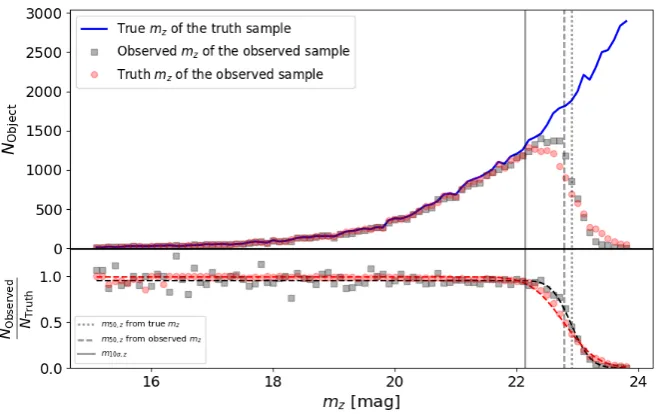
“gold" sample in Section2.2. The simulation is divided into fields of 0.53 deg2, with characteristic quantities like the image depth and seeing matching those of the DES-SV patches. SExtractor is applied to the simulated images with identical DES-SV settings. We select objects withmagerr_auto<0.218 mag inz(5σ signifi-cance), derive their observed magnitude distribution, and compare it to the truth magnitude distribution of all input truth objects (see illustration about the procedure in FigureA1). The ratio between the two is well described by EquationA1. The derivedm50andw

are tightly related to the depth of the image as shown in Figure A2. We also perform the analysis with the Balrog simulation

(Suchyta et al. 2016), which inserts simulated objects into real DES-SV images. The results are similar.

To further verify the derived relations, we stack high quality images from the DES Supernovae survey (with a total exposure time of∼1000s) to mimic main survey depth. Thez-band depth of the stacks ranges from 21.5 mag to 22.5 mag, comparing to>24 mag coadding all eligible exposures. We compare the object counts in this set of coadds and the full coadds to evaluatem50andw(also

shown in Figure A2).

Them50appears to be 0.1 - 0.4 mag deeper than the simulation

relations. The effect is consistent with themag_autobiases shown in Z16. In this test, we compare to the observed Kron magnitudes rather than the "truth" magnitudes (which is not known) from the deeper stack. Z16 shows that the observed Kron magnitudes are fainter by 0.1 to 0.4 mag comparing to the "truth" magnitudes at< 24 mag.

FigureA2indicates that the amplitude of the complementary error function is lower than 1 in UFigand Balrog. This is mostly

caused by the same photometry measurement bias discussed above (another effect is the blending of truth objects, which causes incom-pleteness at a<2% level). Objects are measured fainter by the Kron magnitude. Compared to the truth magnitude distribution, the ob-served magnitude distribution is systematically shifted to the fainter side (see this effect in FigureA1). The result is that the observed magnitude distribution is always lower than the truth distribution, and the amplitude of the fitted completeness function is below 1. This shift and the resulting amplitudes of the completeness func-tion are not of interest in this paper. We explicitly assumes the am-plitudes of the completeness function to be 1.

We notice hints that the completeness function in galaxy clus-ters are different from that of the fields, possibly because of

blend-11 _{Magnitude with magerr_auto=0.108. For a flux measurement at a}

Figure A1.This figure demonstrates our procedure for evaluating completeness function with the UFigsimulation. We model the difference between the

observed magnitude distribution (gray squares in the upper panel) of observed objects and the true magnitude distribution of all truth objects (solid blue line in the top panel). We model the ratio between the observed magnitude distribution and the truth magnitude distribution (gray squares in the lower panel) with a complementary error function (black dashed line). For comparison, we also show ratios between the truth magnitude distributions of the observed and the truth objects (red circles) and the complementary error function fitted model (red dashed line).

ing and larger galaxy sizes. We test the effect with simulated objects (Balrogsimulation,Suchyta et al. 2016) inserted into RedMaPPer

clusters (Rykoffet al. 2016) selected in DES-SV data. We see evi-dence that them50inside galaxy clusters shift by∼0.1 mag

com-paring to fields of equivalent depth (FigureA3). As the sample of simulated galaxies is small, we are unable to characterize the distri-bution of the shifts and hence do not attempt to correctm50in this

paper.

A3 Completeness Limits of the RSLF Analyses

We determine the magnitude limits of the RSLF analyses accord-ing to the completeness functions. We perform the analyses only with galaxies brighter than the following limit:mlim=m50−2

√ 2w. The cut ensures detection probability above 99.8% ×λ for the selected galaxies, according to our fitted completeness function model (EquationA1). Note that the completeness limit is close to the 10-sigma total magnitude limit, which means galaxies above the completeness limit shall have total magnitude measured with significance level above or close to 10σ, and hence above surface brightness detection limit set at the detection (1.5 sigma in SEx-tractor setup), and therefore any surface brightness selection effects should be negligible.

If the cluster region completeness functions follow different relations as discussed above, the magnitude cut still ensures high detection probability (lower limit of 99%×λinstead of 99.8%×λ).

For all of thez<0.4 clusters,mlimis more than 2 mag fainter

than the characteristic magnitude measured inHansen et al.(2009). This is also true for more than 2/3 of the clusters atz>0.4. The

cluster sample size drops steeply above redshift 0.7, and most of the complete clusters are located in the DES deep supernovae fields. As the galaxy samples are highly complete, we do not correct detection probability in this paper.

Because theg,r,i,z-band observations are performed inde-pendently, one may wonder if the image depth in the bluer bands is sufficient for computing colors. For example, thei-band band ob-servation of an object detected inzmay be too shallow that it does not have validi-band photometry measurement. We confirm that af-ter applying the z-band magnitude limit cut (mag_auto_z<mlim),

99.5% and 99.6% of the cluster region objects are detected inr

and i respectively. 98.3% or 99.2% of the objects have good r

ori-band photometry measurement (magerr_autoabove 3σ, i.e.,

magerr_auto<2.5/ln10/3). We conclude that the DES multi-band

data are sufficiently deep for red galaxy selection.

APPENDIX B: CLUSTER INFORMATION

REFERENCES

Allen S. W., Evrard A. E., Mantz A. B., 2011,ARA&A,49, 409 Andreon S., 2008,MNRAS,386, 1045

Balogh M. L., Morris S. L., 2000,MNRAS,318, 703 Balogh M. L., Navarro J. F., Morris S. L., 2000,ApJ,540, 113 Behroozi P. S., Wechsler R. H., Conroy C., 2013,ApJ,770, 57

Bergé J., Gamper L., Réfrégier A., Amara A., 2013,Astronomy and Com-puting,1, 23

Berlind A. A., Weinberg D. H., 2002,ApJ,575, 587

Bertin E., 2011, in Evans I. N., Accomazzi A., Mink D. J., Rots A. H., eds, Astronomical Society of the Pacific Conference Series Vol. 442, Astronomical Data Analysis Software and Systems XX. p. 435 Bertin E., Arnouts S., 1996,A&AS,117, 393

Blanton M. R., Roweis S., 2007,AJ,133, 734 Bleem L. E., et al., 2015,ApJS,216, 27 Boselli A., Gavazzi G., 2014,A&ARv,22, 74

Bower R. G., Lucey J. R., Ellis R. S., 1992, MNRAS,254, 589 Bruzual G., Charlot S., 2003,MNRAS,344, 1000

20 21 22 23 24

m

20 21 22 23 24 25

m

z

(a)

UFIG fitted relation

(1.010± 0.004)×

m

20 21 22 23 24

m

−0.2 0.0 0.2 0.4

m

z

R

esi

d)

al

(b)

20 21 22 23 24

m

0.0 0.1 0.2 0.3 0.4 0.5

w

UFIG fi((ed rela(ion

(0.021+ 0.002),

m

Balrog SN restack

20 21 22 23 24

m

0.6 0.7 0.8 0.9 1.0 1.1 1.2

λ

(d)

UFIG Average 0.9423± 0.0004

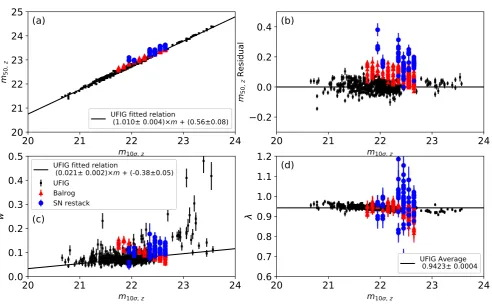
Figure A2.This figure shows the relations between completeness function parameters and the image depth, characterized by the 10σlimiting magnitude. Panel (a) shows the dependences ofm50, the 50% completeness magnitude, on image depth from the UFig(black points), Balrog(red triangles) simulations and the

SN restack data (blue circles). Panel (b) shows them50residuals of the three data sets from the UFig relation. The relation derived with the UFigsimulation

generally agrees with the data from the Balrogsimulation. Them50values evaluated from re-stacking deep supernovae data appear to be 0.1-0.2 mag deeper,

but the differences can be explained by the Kron magnitude bias shown in Z16. Panel (c) shows the dependences ofw, the steepness of the detection drop-out rate, on image depth. We use the UFigsimulation relations for bothm50andwin this paper. We notice that the completeness function amplitudes from

simulations appear to be lower than 1 as shown in panel (d), but it is mostly caused by the differences between observed and truth magnitudes (see a discussion in SectionA2).

23.5 24.0 24.5

m

−0.4 −0.2 0.0 0.2 0.4

m

z

,B

K

G

-m

z

,C

lu

st

er

0 5 10 15 20 −0.4

−0.2 0.0 0.2 0.4

Figure A3.We evaluate them50 parameters (50% completeness

magni-tudes) for cluster and for field regions of the same depth with the Bal

-rogsimulation. Them50of a cluster region is potentially shallower by∼0.1

mag compared to a same-depth field region potentially because of blending in the cluster region.

0.0 0.2 0.4 0.6 0.8 1.0 1.2

Redshift

0 1 2 3 4 5 6 7

m

,z

−m

*,z

[m

ag

]

Figure A4.For each cluster, we derive a completeness limit,mlimfrom the

completeness function. Atz<0.4 , all of the DES XCS-SV clusters are

complete tom∗_z+2 mag and beyond. This is also true for more than 2/3 of

the clusters atz>0.4. Incomplete clusters ofmlimbelowm∗z+2 mag are not

included in this paper’s analyses. The scatters ofmlimare caused by DES