A Novel Solution Approach using Linearization Technique for Nonlinear Programming Problems

A Novel Solution Approach using Linearization

Technique for Nonlinear Programming Problems

Mustafa Sivri

Department of Mathematical Engineering Yildiz Technical University

Istanbul, Turkey

Inci Albayrak

Department of Mathematical Engineering Yildiz Technical University

Istanbul, Turkey

Gizem Temelcan

Department of Computer Programming Istanbul Aydin University

Istanbul, Turkey

ABSTRACT

In this paper, a novel solution approach for solving the non-linear programming (NLP) problems having m nonlinear alge-braic inequality (equality or mixed) constraints with a nonlin-ear algebraic objective function in n variables using lineariza-tion technique is presented. This approach performs successive increments to find a solution of the NLP problem, based on the optimal solutions of linear programming (LP) problems, satis-fying the nonlinear constraints oversensitively. In the proposed approach, the original problem is converted to the LP prob-lem using increments in the linearization process and the im-pact of computational efficiency makes the performance of the solution well. It is presented that how the solution approach can be applied to solve the illustrated examples from the literature.

General Terms

Computational Mathematics, Optimization

Keywords

Linear Programming, Incremental Technique, Taylor Series, Lin-earization Algorithm

1. INTRODUCTION

Constructing a mathematical model for real life problems is an im-portant issue in optimization theory. Optimization problems can be classified according to the nature of the objective function and con-straints. An optimization problem can be defined as min (or max) of a single (or multi) objective function, subject to (or not to) single (or multi) nonlinear (or linear) inequality (or equality or mixed) con-straints. If all objective function(s) and constraint(s) are linear, then the problem is known LP problem. NLP problems are a special ver-sion of LP, i.e., the objective function and/or constraint(s) are non-linear, that is called general NLP problems. LP or NLP problems optimize the objective function(s) subject to finite number of con-straints, considering whether subject to non-negativity constraints or not.

There is no effective method for solving the general NLP problems like simplex method in LP. When the number of variables or con-straints increases, solving NLP problems numerically needs huge computational efforts by using special optimization algorithms [6]. Since 1951, there has been great progress for solving NLP prob-lems. Hestenes [9] proposed augmented Lagrangian methods for solving equality constrained problems. This approach was extended in [12] to the constrained optimization problem with both equality and inequality constraints. Sannomiya et al. [13] proposed an ef-fective method even if there is no feasible solution satisfying the approximate linear constraints.

Linearization methods can be used converting a NLP problem into a LP problem. In this process, extra variables and constraints are in-troduced to construct the original problem. Various methods have been proposed in the literature by linearizing a NLP problem [14], [11]. Sequential Linear Programming (SLP) which is one of the direct methods solves NLP problems approximately, and uses a se-ries of LP problems generated by using first order Taylor sese-ries expansions of objective functions and constraints. Byrd and No-cedal [3] have presented a new active-set, trust-region algorithm for large-scale optimization using SLP techniques to solve the NLP problems approximately.

This iterative approach constructs different optimization problems corresponding to the parameter related with arbitrary points which are chosen satisfying the constraints.

In this paper, a novel solution approach for solving general NLP problems, havingmnonlinear (or linear) algebraic inequality (or equality or mixed) constraints with nonlinear (or linear) objective function innvariables is presented. The original problem is con-verted to the LP problem using increments in the linearization pro-cess and the impact of computational efficiency makes the perfor-mance of the solution well.

This paper is organized as follows: Section 2 presents brief required information used in this work. In Section 3, the proposed approach is handled. Section 4 and Section 5 consist of numerical examples and conclusions, respectively.

2. PRELIMINARIES

In this section, required information is presented.

DEFINITION 1. A general constrained NLP problem can be de-fined as follows:

min f(x)

s.t.

gi(x) =bi, i= 1,2, ..., p

gj(x)≤bj, j=p+ 1, ..., m

(1)

wherex= [x1, x2, ..., xn]∈Rnis a vector,gi :Rn→ R,(i=

1,2, ..., p),gj : Rn → R,(j =p+ 1, ..., m). In (1), if the

ob-jective function and all constraints are linear, it is known as an LP problem.

DEFINITION 2. [5] Any point xsatisfying the constraints is called the feasible point. The set of all feasible points is called the feasible set such thatX = {x ∈ Rn _{: g}

i(x) = bi,(i =

1,2, ..., p), gj(x)≤bj,(j=p+ 1, ..., m)}.

DEFINITION 3. An optimal solutionx∗

to a LP problem is a feasible solution with the smallest objective function value for a minimization problem.

DEFINITION 4. A pointxin the feasible setXis said to be an interior point ifXcontains some neighborhood ofx.

DEFINITION 5. After converting NLP problem to LP problem, the obtained solution is called a linearization point.

3. THE PROPOSED APPROACH

A novel solution approach for solving general NLP problems, hav-ing m nonlinear (or linear) algebraic inequality (or equality or mixed) constraints with nonlinear (or linear) objective function in nvariables is presented. The iterations present reasonable progress to convert the NLP problem using successive linearization process by means of Taylor series expansions.

Step 1 Load the NLP problem havingmnonlinear constraints with a nonlinear objective function innvariables as given in (1).

Step 2 Construct Lagrangian function

L(xk, λi, λj) =f(xk) +P_iλi(gi(xk)−bi)

+P

jλj(gj(xk)−bj)

(2)

wherek= 1, ..., n;i= 1,2, ..., p;j=p+ 1, ..., m.

Step 3 Construct a nonlinear system obtained from (2).

∂L

∂xk = 0, k= 1, ..., n

∂L

∂λi = 0, i= 1, ..., p

λj(gj(x1, ..., xn)−bj) = 0, j=p+ 1, ...., m

(3)

Step 4 Choose any initial arbitrary nonzero point(xk, λi, λj), k =

1, ..., n;i= 1, ..., p;j=p+ 1, ..., m.

Step 5 Linearize each equation in (3) by expanding Taylor series at the chosen point.

Step 6 Construct a linear system as follows:

∂L

∂xk

L= 0, k= 1, ..., n ∂L

∂λi

L= 0, i= 1, ..., p

λj(gj(x1, ..., xn)−bj)

L= 0, j=p+ 1, ...., m

(4)

where the subscriptL is used to show the linearization, and solve the system in (4).

Step 7 Analyze the solution of the system in (4):

If there is a solution as¯x= (¯x1, ...,x¯n), go to Step 8.

Else, go to Step 4.

Step 8 Check the types of constraint of (1):

If they are mixed or equality constraints, go to Step 9. If they are inequality constraints, go to Step 13.

Step 9 Linearize each equation in (3) by expanding Taylor series at¯x.

Step 10 Solve the reconstructed linear system.

Step 11 Analyze the solution obtained in Step 10:

If there is a solution asx= (x₁, ..., x_n), go to Step 12. Else, go to Step 4.

Step 12 Check successive two objective function values:

For a given >0if|f(¯x)−f(x)| ≤, then it is a solution of the NLP problem in (1) and STOP.

Else, assignxtox¯, and go to Step 9.

Step 13 Check the solutionx¯:

If it satisfies all constraints of (1) individually, go to Step 14.

Else, linearize each equation in (3) by expanding Taylor series atx¯, and go to Step 6.

Step 14 Introduce new variablesxˆ = (ˆx1, ...,xˆn)by making

incre-ments

ˆ

xk= ¯xk+uk−vk (5)

whereuk, vk,(k= 1, ..., n)are nonnegative variables defined

as0≤uk≤1and0≤vk≤1.

Step 15 Substitutexˆgenerated in (5) into objective function and con-straints of (1).

Step 16 Linearize new objective function and each constraint obtained in Step 15 by expanding Taylor series.

Step 17 Construct a LP problem by adding new constraints min fL(u1, ..., un, v1, ..., vn)

s.t.

gLj(u1, ..., un, v1, ..., vn)≤bj, j=p+ 1, ...., m

0≤uk≤1, k= 1, ..., n

0≤vk≤1, k= 1, ..., n

(6)

and solve (6).

Step 18 Check the solution of (6):

If there is a feasible solution, go to Step 19. Else, go to Step 4.

If allu, vare zero,ˆxis a solution for the NLP problem (1) and STOP.

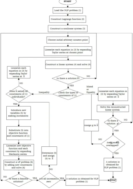
Else, determineˆx. Assignxˆtox¯, and go to Step 14. The flow chart of the proposed approach is given in Figure1.

Fig. 1. The flow chart of the proposed approach

4. NUMERICAL EXAMPLES

Example 1 [2]Solve the NLP problem min (x1−2)2+ (x2−2)2

s.t. x2

1+x22−1 = 0

x2

2−x1≤0

(7)

using the proposed approach where= 10−5_.

Step 1-2. Load the NLP problem (7) and construct Lagrangian function:

L(x1, x2, λ1, λ2) = (x1−2)2+ (x2−2)2

+λ1(x21+x22−1) +λ2(x22−x1).

(8)

Step 3. Construct the following nonlinear system obtained from (8).

2(x1−2) + 2λ1x1−λ2= 0

2(x2−2) + 2λ1x2+ 2λ2x2= 0

x2

1+x22−1 = 0

λ2(x22−x1) = 0.

(9)

Step 4. Choose any initial arbitrary nonzero point:x1 = 3, x2 =

3, λ1= 1,λ2= 1.

Step 5-6. Linearize each equation in (9) by expanding Taylor series at chosen point, and construct the following linear system.

4x1+ 6λ1−λ2= 10

6x2+ 6λ1+ 6λ2= 16

6x1+ 6x2= 19

−x1+ 6x2+ 6λ2= 15

(10)

Step 7.The solution of (10) is obtained as x1 = 4.5455, x2 =

−1.3788, λ1=−0.5909,λ2= 4.6364.

Summarized results of Example 1 using the proposed approach is given in Table 1. Basirzadeh also solved this problem in [2]. The comparison of solutions is presented in Table 2. The optimal solution obtained by the proposed approach satisfies the equality constraint of (7) oversensitively, however it is not verified with Basirzadeh’s solution.

Table 1. Iteration Results of Example 1 Iterations x1 x2 f(x1, x2)

1st 4.5455 -1.3788 17.8959 2nd 2.385 -0.682 7.3413 3rd 1.8908 1.3679 0.4115 4th 1.6591 0.063 3.8682 5th 1.0905 1.0966 1.6433 6th 0.5921 0.9577 3.0686 7th 0.633 0.7926 3.3265 8th 0.6182 0.7862 3.3827 9th 0.6181 0.7861 3.3832 10th 0.6181 0.7861 3.3832

Table 2. The Comparison of Solutions of Example 1

Basirzadeh’s Approach Proposed Approach

x1 0.7070 0.6181

x2 0.7070 0.7861

z 3.3437 3.3832

Optimal solution of the NLP problem (9) isx∗

1 = 0.6181, x∗2 =

0.7861and the optimal value isz∗_{= 3.3832.}

Example 2 [4]Solve the NLP problem

max 3x3 1+ 2x32

s.t. x2

1+x 2

2−16≤0

x1−x2−3≤0

(11)

using the proposed approach where= 10−5_.

Step 1-2. Load the NLP problem (11) and construct Lagrangian function:

L(x1, x2, λ1, λ2) =−3x31−2x 3

2+λ1(x21+x 2 2−16)

+λ2(x1−x2−3).

Step 3. Construct the following nonlinear system obtained from (12).

−9x2

1+ 2λ1x1+λ2= 0

−6x2

2+ 2λ1x2−λ2= 0

λ1(x21+x22−16) = 0

λ2(x1−x2−3) = 0.

(13)

Step 4. Choose any initial arbitrary nonzero point:x1 = 5, x2 =

1, λ1= 1,λ2= 2.

Step 5-6. Linearize each equation in (13) by expanding Taylor se-ries at chosen point, and construct the following linear system.

88x1−10λ1−λ2= 215

10x2−2λ1+λ2= 4

10x1+ 2x2+ 10λ1= 52

2x1−2x2+λ2= 8

(14)

Step 7.The solution of (14) is obtained as

x1= 2.75, x2= 0.5161, λ1= 2.3468, λ2= 3.5323. (15)

Step 8-13. Check if the solution obtained in (15), providing all the constraints in (11).

It is seen that this solution satisfies the constraints individually. Step 14. Introduce new variablesxˆ1,xˆ2by making increments

ˆ

x1= 2.75 +u1−v1

ˆ

x2= 0.5161 +u2−v2 (16)

whereu1, u2, v1, v2are nonnegative variables.

Step 15-17. Substituteˆx1,xˆ2generated in (16) into objective

func-tion and constraints of (11), linearize new objective funcfunc-tion and each constraint by expanding Taylor series, and construct the fol-lowing LP problem by adding new constraints

max 68.0625(u1−v1) + 1.5982(u2−v2)

5.5(u1−v1) + 1.0322(u2−v2)≤8.1711

(u1−v1)−(u2−v2)≤0.7661

0≤u1≤1; 0≤u2≤1

0≤v1≤1; 0≤v2≤1

(17)

and solve (17).

Step 18-19. The solution of (17) isu1 = 1, v1= 0, u2 = 1, v2=

0. Becauseu1, u2, v1, v2are different from zero,xˆ1= 3.75,ˆx2=

1.5161are determined.xˆ1,xˆ2 are assigned tox¯1 = 3.75,x¯2 =

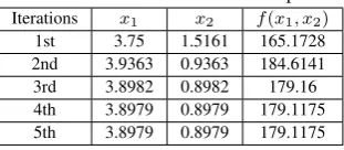
1.5161, respectively. Then, go to Step 14. Until allu1, v1, u2, v2

become zero, the process is continued from Step 14 to Step 19. The proposed approach is applied to the problem solved in [4]. The approach is more efficient than Chis¸ and Cret’s approach for max-imizing (11). Summarized results and the comparison of solutions are shown in Table 3 and Table 4, respectively.

Table 3. Iteration Results of Example 2 Iterations x1 x2 f(x1, x2)

1st 3.75 1.5161 165.1728 2nd 3.9363 0.9363 184.6141 3rd 3.8982 0.8982 179.16 4th 3.8979 0.8979 179.1175 5th 3.8979 0.8979 179.1175

Optimal solution of the NLP problem (11) isx∗1 = 3.8979, x

∗

2 =

0.8979and the optimal value isz∗_{= 179.1175} .

Table 4. The Comparison of Solutions of Example 2 Chis and Cret’s Approach Proposed Approach

x1 3.875 3.8979

x2 0.875 0.8979

z 175.8965 179.1175

5. CONCLUSION

In this paper, a novel solution approach for solving general NLP problems, havingmnonlinear (or linear) algebraic inequality (or equality or mixed) constraints with nonlinear (or linear) objective function innvariables is presented. This solution approach is ap-plied according to structure of constraints:

This approach performs successive LP problems using incre-ments after solving linear system(s) obtained from Lagrangian function to find a solution of the NLP problem subject to in-equality constraints.

This approach also finds a solution of the NLP problem un-der mixed or equality constraints. The solution is based on the solutions of linear systems obtained from Lagrangian function. After performing linearization approach at any initial arbitrary nonzero point for each type of structure of constraints, the obtained solution of the original NLP problem satisfies the constraints sen-sitively while making the objective function min or max.

6. REFERENCES

[1] Inci Albayrak, Mustafa Sivri, and Gizem Temelcan. A new it-erative approach for solving nonlinear programming problem. New Trends in Mathematical Sciences, 6(2):68–77, 2018. [2] H Basirzadeh, AV Kamyad, and S Effati. An approach for

solving nonlinear programming problems.Korean Journal of Computational & Applied Mathematics, 9(2):547–560, 2002. [3] Richard H Byrd, Nicholas IM Gould, Jorge Nocedal, and Richard A Waltz. An algorithm for nonlinear optimization using linear programming and equality constrained subprob-lems.Mathematical Programming, 100(1):27–48, 2003. [4] Codrut¸a Chis¸ and F Cret¸. Solving nonlinear programming

problems by linear approximations. 2005.

[5] Edwin KP Chong and Stanislaw H Zak.An introduction to optimization, volume 76. John Wiley & Sons, 2013. [6] Gerard Cornuejols and Reha T¨ut¨unc¨u.Optimization methods

in finance, volume 5. Cambridge University Press, 2006. [7] Philip E Gill and Elizabeth Wong. Sequential quadratic

pro-gramming methods. In Mixed integer nonlinear program-ming, pages 147–224. Springer, 2012.

[8] Chuan-Hao Guo, Yan-Qin Bai, and Jin-Bao Jian. An im-proved sequential quadratic programming algorithm for solv-ing general nonlinear programmsolv-ing problems. Journal of Mathematical Analysis and Applications, 409(2):777–789, 2014.

[9] Magnus R Hestenes. Multiplier and gradient methods. Jour-nal of optimization theory and applications, 4(5):303–320, 1969.

[11] Ming-Hua Lin, John Gunnar Carlsson, Dongdong Ge, Jian-ming Shi, and Jung-Fa Tsai. A review of piecewise lineariza-tion methods.Mathematical problems in Engineering, 2013, 2013.

[12] R Tyrrell Rockafellar. Augmented lagrange multiplier func-tions and duality in nonconvex programming.SIAM Journal on Control, 12(2):268–285, 1974.

[13] Nobuo Sannomiya, Yoshikazu Nishikawa, and Yoshikazu Tsuchihashi. A method for solving nonlinear programming problems by linearization.The transactions of the Institute of Electrical Engineers of Japan. C, 97(1-2):12–18, 1977. [14] Claus Still and Tapio Westerlund. A linear