A State Transition MIP Formulation for the Unit
Commitment Problem
Semih Atakan, Guglielmo Lulli, Suvrajeet Sen,
Member
Abstract—In this paper, we present the state-transition formu-lation for the unit commitment (UC) problem. This formuformu-lation uses new decision variables that capture the state transitions of the generators, instead of their on/off statuses. We show that this new approach produces a formulation which naturally includes valid inequalities, commonly used to strengthen other formulations. We demonstrate the performance of the state-transition formulation and observe that it leads to improved solution times especially in longer time-horizon instances. As an important consequence, the new formulation allows us to solve realistic instances in less than 12 minutes on an ordinary desktop PC, leading to a speed-up of a factor of almost two, in comparison to the nearest contender. Finally, we demonstrate the value of considering longer planning horizons in UC problems.
Index Terms—Mixed-integer linear programming, unit com-mitment
I. INTRODUCTION
Every day regional electricity networks deliver millions of kilowatt-hours of energy from generating units to consumers. These production requirements vary by season, day-of-the week, and hour. As a result, efficient scheduling of electricity production continues to attract significant attention from both industry and academia in the form of the so-called unit commitment (UC) problem. Such a model must recommend which generators to use, and how much they should produce so that demand over a planning horizon is met, while obeying certain operating rules, maintenance schedules, and in some instances, transmission capacity requirements. The goal is to obtain the most cost-effective operating schedule over a large set of generators, and ensure that the demand is completely fulfilled during the planning horizon.
With the liberalization of the energy industry, the introduc-tion of energy market concepts and privatizaintroduc-tion, the role of the UC models has changed [1]. UC problems are solved by a variety of constituents of the electric power industry, each for a different purpose. A specific utility may solve the UC problem for the purposes of planning production within their delivery area. Their costs also helps them to place bids in the Independent System Operator (ISO) exchange market. On the other hand, the ISO solves its UC model to decide which bids to accept and to set prices that will be paid to the suppliers. These problems are much larger because they involve multiple suppliers, and with a number
S. Atakan & S. Sen are with Daniel J. Epstein Department of Industrial and Systems Engineering, University of Southern California, Los Angeles, USA (e-mail: [email protected]; [email protected]).
G. Lulli is with the Department of Management Science, Lancaster Uni-versity, Lancaster, United Kingdom (e-mail: [email protected])
This research has been supported by the NSF (ECCS-1548847).
of generating units in the order of thousands. Providing high-quality solutions to these realistic problems is computationally very demanding but has the potential for significant reduction in costs. A 2011 report of the Federal Energy Regulatory Commission (FERC) suggests that savings approaching a $100 million annually can be expected by replacing heuristics with methods that seek optimal solutions (see [2]). Consequently, developing solution methods that can achieve high-quality solutions in a short amount of time has been the focus of significant research over the last several decades.
Many optimization methods have been proposed to solve the UC problem. For example, we mention branch-and-bound methods [3], dynamic programming approaches [4], La-grangian relaxation methods [5], [6], and unit decommitment [7], among others. For a detailed review, the reader is referred to [8], [9]. In recent years, mixed-integer programming (MIP) has emerged as a popular tool for solving UC problems. A discussion on its merits and drawbacks (with respect to La-grangian relaxation) were given in [10]. The popularity of MIP led to significant advances in the mathematical description of specific features of the UC problem. For instance, [11] have identified the convex hull for a minimum up/downtime polytope, [12] provided the convex hull of generation lim-its and this minimum up/downtime polytope, [13] provided strengthened inequalities of a ramping polytope, and [14] provided the convex hull of a two-period ramping polytope.
Nevertheless, it is well known that in general, mixed-integer programs areN P-hard, and solving problems of realistic size, involving thousands of generators, over several time periods, remains challenging. Moreover, the introduction of variable energy resources (e.g., wind and solar) leads to circumstances in which predictions from deterministic models are subject to significant errors. In order to accommodate such challenges, there have been recommendations that UC models should be solved using either the stochastic or the robust UC formula-tions (see, e.g., [15] and [16], respectively). In either case, the speed with which large scale deterministic UC models can be solved becomes important.
solution methods, leading to faster solution times without mod-ifying the underlying optimization methodologies. Second, we show that the use of state-transition variables naturally lead to certain facet-defining constraints in our problem-of-interest. This contrasts with the majority of other formulations available in the literature which often require the addition of further in-equalities in order to generate the same strong (facet-defining) valid inequalities. Finally, we perform a computational study to demonstrate the behaviors of the new, and two relatively recent and well regarded benchmark formulations. This study sheds further light on the classes of instances for which the new formulation outperforms the contenders.
II. FORMULATING PRODUCTION AND OPERATIONS IN UNIT COMMITMENT
Beginning with the MIP formulation of [19], a plethora of mathematical formulations have been proposed in the literature to solve instances of the UC problem. These have extended the work of Garver in several directions. The mathematical modeling has been enriched with many additional aspects of the problem, and made it more realistic. For instance, several operational and technological restrictions have been included in the UC formulations, and significant efforts have been made in improving the formulation of operating costs. Other objectives have also been considered, such as the minimization of no load or turn off costs, maximization of social welfare, or maximization of the profit of generator companies (see [20]). In addition to refining the mathematical modeling, a lot of academic research in this field has been devoted to developing strong MIP formulations, so that real-scale instances of the problem can be handled with advanced MIP solvers.
As considered in [13] and [21], the core requirements of a UC problem involves the following components:
• minimum and maximum production restrictions, • start up / shut down limits, and ramping restrictions, • minimum up/downtime requirements,
• demand and reserve requirements (modeled as stand-by capacities)
• start up costs (defined as step-functions of the generators’ idle times) and production costs (defined as piecewise-linear convex functions of the production amounts)
We adopt this core setup although other advanced requirements (e.g., transmission, power flow, line flow, and voltage limits, etc) are typically accommodated in realistic applications [22]. The purpose of our study will be to compare three alternative MIP formulations, which consider the above listed modeling considerations of a UC problem.
To begin our discussion, we present a prototypical MIP formulation of this UC model. Given a set of generatorsG, and hourly discretized time periodsT, we introduce the following decision variables that are ubiquitous in the literature:
xg,t: State variable (1 ifgis operational at time t, 0 otherwise),
sg,t/ zg,t: Start up / shut down variable (1 if g is turned on / off at timet, 0 otherwise),
pg,t: Amount of production byg at timet.
The state variables are fundamental for the scheduling of generators. The start up / shut down variables are used to formulate the operating costs of the generators, whereas the production variables determine the dispatch amounts. In what follows, a vector of variables of the same type (say
xg,t,∀g∈ G, t∈ T) will be typed in bold (sayx).
The objective of the mathematical formulation is to compute a power generation plan which satisfies production require-ments along with operational constraints. The total opera-tional costs include both the production and the start up costs. Both of these costs are nonlinear, in general. In our prototypical formulation, these costs are represented with the following (nonlinear) functions:Fg(·), for the start up costs, and Vg(·), for the production costs. The argument of the cost functions are respectively i- and j-dimensional vectors xg,[t] = (xg,t−i. . . xg,t) and pg,[t] = (pg,t−j. . . pg,t), for
some i ≥ 0 and j ≥ 0. This indicates the dependency of the costs, respectively, on the past states and the production levels of the generator.
A prototypical formulation is given below:
min X
g∈G
X
t∈T
Fg(xg,[t]) +Vg pg,[t]
s.t. xg,t−xg,t−1=sg,t−zg,t ∀g∈ G, t∈ T, (1a)
pg,t≥
¯
Cgxg,t ∀g∈ G, t∈ T, (1b)
pg,t≤Cgxg,t¯ ∀g∈ G, t∈ T, (1c) P
g∈G pg,t≥dt ∀t∈ T, (1d)
(x, s, z, p)∈ D (1e)
(x, s, z)∈ {0,1}3|G||T |, p≥0. (1f)
Above, dt is the demand for electricity at period t,Cg¯ is the maximum generation capacity and
¯
Cgis the minimum required production amount when the generator is operational.
The constraints (1a)links thesg,t andzg,t variables to the state variables. Indeed, these variables are completely deter-mined once the values of x are known. They are introduced exclusively to capture the transition of a generator between idle and operational state, and to formulate the operating costs of a generator. Constraints (1b) and (1c) model the lower and upper bounds, respectively. Constraints (1d) impose that the production levels must meet the demand for energy at any period. Finally, constraints (1e) state that a feasible solution must belong to the polyhedronD, which will be described in detail in the following paragraphs.
The integrality requirements on the (s,z) variables can be relaxed without invalidating the formulation. This observation was exploited by [23] to formulate the UC problem with inte-grality restrictions on xalone. However, the assumed benefit of using considerably smaller number of binary variables does not necessarily lead to superior computational performance, as observed by [13]. This is due to improved formulations and more robust MIP solvers.
Before proceeding further, we define the following notation which will be used throughout this paper:
¯
Rg/
¯
Rg: Ramp-up / ramp-down limit,
¯
Sg/
¯
Sg: Start up / shut down limit,
The data of a typical UC instance usually obey the following relations: Cg¯ ≥Rg¯ ≥Sg¯ ≥
¯
Cg >0 and Cg¯ ≥
¯
Rg ≥
¯
Sg ≥
¯
Cg>0, ∀g∈ G. We assumeU Tg ≥1andDTg≥1to avoid cases where the generator is simultaneously turned on and off.
A. Formulating the components
The majority of the UC formulations in the literature can be perceived as extensions of the prototypical formulation (1). These formulations differ in the way they define oper-ational constraints, nonlinear objective functions, and produc-tion quantities. Nonetheless, the state of a generator is almost unanimously determined by(x,s,z)variables, as first defined in the seminal work of [19]. In this section, we will identify all the components that go into modeling different considerations in a UC problem. In the next section, we will integrate them together into specific formulations, which correspond to the studies of [13] and [21]. In what follows, we will allow nonpositive indices of the decision variables to make it explicit that a solution of the problem might depend on the past states of the generators. In the actual implementation, we fix such variables to their realized values according to the available past data.
a) Formulating production quantities: An integral part of a UC formulation is the description of feasible produc-tion schedules that consider demand and operating reserve requirements along with minimum/maximum production re-strictions. In the UC literature, the predominant choice for formulating production amounts has been through the pg,t
variables. These variables are intuitive and simple, however, they may inadvertently introduce unneeded complexity into an MIP formulation. In particular, the presence of minimum production restrictions (1b) implicitly alters the continuous nature of these variables, leading to semi-continuous variables that must either equal 0 or lie within the range [
¯
Cg,Cg¯ ]. To avoid this, the following variables can be used in lieu ofpg,t:
p0
g,t: The production amount beyondCg¯ provided by
gen-eratorg at timet.
This new variable only accounts for the variable portion of production. Thefixedportion of production (i.e., the minimum production amount) is associated with the state variables as
¯
Cgxg,t. Combining these, we can form the linear mapping
pg,t → (p0
g,t +Cgxg,t¯ ) which can be used to infer the
total production amount. Moreover, after applying this map-ping throughout the formulation, one can observe that the minimum production constraints are immediately satisfied. Consequently, |G| × |T | constraints in (1b) can be omitted from the formulation without sacrificing its fidelity.
The idea to treat the minimum and the variable production amounts separately was originally considered in [19]. Over the decades, this idea had been set aside, until the study of [21], who provided a modern look at this representation. Along with the use of p0
g,t variables, their study provides tighter
descriptions of the production capacity restrictions which will be presented later in this section.
We continue with formulating the operating reserves. These requirements are stand-by capacities that must be kept ready to provide for unplanned outages of generating units. System
operators use operating reserves to maintain system reliability and to ensure that the supply-demand balance is achieved seamlessly. [22] and [24] provide examples on how to for-mulate these requirements. To demonstrate, we introduce the following alternate sets of variables:
¯
pg,t: The maximum generation amount that g can supply at timet,
rg,t: The generation amount that g can supply at time t
for reserve requirements.
Both of these variables, by themselves, capture all the neces-sary information to formulate the reserve requirements. Indeed, the relation between these variables can be described with the mapping pg,t¯ →(pg,t+rg,t).
In view of the discussion in this section, we provide two alternatives for formulating production, which respectively appeared in the state-of-the-art formulations of [13] (see constraints (2)-(3)) and [21] (see (4)-(6)). We begin with the former, where the (pg,t,pg,t¯ ) variables are used and the followingproduction limitsare imposed for allg∈ G, t∈ T:
¯
Cgxg,t ≤ pg,t ≤ pg,t¯ ≤ Cgxg,t¯ + ( ¯
Sg−Cg¯ )zg,t+1. (2)
The above constraints ensure that (i) if the generator is idle (i.e., xg,t = 0), the production amounts cannot be positive,
(ii) if the generator is operational (i.e., xg,t = 1), the minimum production requirements and capacity restrictions must be obeyed, and (iii)if the generator is scheduled to be turned off in the next period (i.e.,zg,t+1 = 1), the maximum generation amount cannot exceed the shut down limit. For
t = |T |, the zg,t+1 variable on the right-most inequality in (2) is assumed to be 0. The pg,t¯ variables must also be smaller than the start up limit Sg¯ whenever the generator is turned on at time t, however, this requirement will already be satisfied by the ramping inequalities presented in the next section. Finally, letting ρt be the required reserve amount at time t, the following constraints make sure that the reserve requirementsare fulfilled:
P
g∈G pg,t¯ ≥dt+ρt ∀t∈ T. (3)
As an alternative for the above formulation of production, [21] utilize the(p0
g,t, rg,t)variables. As previously stated, the
minimum production constraints are redundant whenp0 g,t
vari-ables are in use, therefore omitted. The following constraints provide a tight description ofproduction limits:
p0g,t+rg,t≤( ¯Cg−Cg¯ )xg,t−( ¯Cg−Sg¯ )sg,t
−max( ¯Sg−
¯
Sg,0)zg,t+1 ∀g∈ G, t∈ T,(U Tg= 1) (4a)
p0g,t+rg,t≤( ¯Cg−Cg¯ )xg,t−( ¯Cg−¯Sg)zg,t+1 −max(
¯
Sg−Sg,¯ 0)sg,t ∀g∈ G, t∈ T,(U Tg= 1) (4b)
p0g,t+rg,t≤( ¯Cg−Cg¯ )xg,t−( ¯Cg−Sg¯ )sg,t
−( ¯Cg−
¯
Sg)zg,t+1 ∀g∈ G, t∈ T, (U Tg>1). (4c)
With respect to constraints (1d), the use of p0
g,t variables
necessitate an update in the demand constraints, as below:
P
g∈G p0g,t+Cgxg,t¯ ≥dt ∀t∈ T. (5)
Finally, the following inequalities ensure that the reserve requirementscan be fulfilled:
P
g∈G rg,t≥ρt ∀t∈ T. (6)
b) Formulating operational and technological restric-tions: In order to compute realistic production schedules, the MIP formulations must take into account the physical limitations of the components of the power systems. Among these limitations, some of the most essential ones are the min-imum up/downtime and ramping restrictions. The minmin-imum up/downtime restrictions ensure that the on/off status of the generators do not change rapidly. Frequent state transitions have several adverse consequences including (i) increased operator stress, (ii) diminished generator life, and (iii) in-creased emission of pollutants during transient periods (see [25]). Such restrictions are quite practical and are included in many commercial tools. To formulate these restrictions, several constraints were proposed in [24], [25], [26]. Following [11], the minimum uptime and downtime constraints are best formulated using the following constraints:
Pt
i=t−U Tg+1sg,i≤xg,t g∈ G, t∈ T, (7a)
Pt
i=t−DTg+1 sg,i≤1−xg,t−DTg g∈ G, t∈ T. (7b)
Observe that when the generator g is operational at time
t, the right-hand side of constraint (7a) is set to 1. In this case, the generator may have been turned on at most once in the last U Tg periods (due to minimum uptime restrictions). On the other hand, if it is idle at time t, it could not have been turned on in the last U Tg time periods, as otherwise it should be operational at time t. Constraint (7b) is just a rewritten version of a similar constraint for the downtime requirements. It has been widely observed that these turn on/off inequalities significantly outperform its contenders [13]. Indeed, [11] showed that constraints (7) define facets of the polytope defined by the minimum up/downtime constraints.
The ramping restrictions limit the maximum change in production between consecutive periods and ensure that the generation requirements can be matched by the electricity production without exceeding the generator limitations over extended periods of time. A basic representation of these
ramping restrictions, in the space of p0
g,t and rg,t variables,
appears below:
p0g,t+rg,t−p0g,t−1≤Rg¯ ∀g∈ G, t∈ T, (8a)
p0g,t−1−p 0
g,t≤Rg¯ ∀g∈ G, t∈ T. (8b)
The above inequalities, by themselves, do not take into account the start up and shut down rates of the generators. Indeed, certain generation limit constraints (such as (4)) must be used in conjunction with (8) to make sure these restrictions are also satisfied.
The ramping inequalities may also be written in the space of pg,t andpg,t¯ variables. Below, we give the formulation of
ramping restrictionsthat appeared in [13].
¯
pg,t−pg,t−1≤Sgsg,t¯ + ¯Rgxg,t−1 ∀g∈ G, t∈ T, (9a)
pg,t−1−pg,t≤
¯
Sgzg,t+ ¯
Rgxg,t ∀g∈ G, t∈ T. (9b)
Constraint (9a) ensures that generatorgcannot ramp up more thanSg¯ if it has just been turned on, or Rg¯ if it remains on at timet. Similarly, constraint (9b) limits the decrease in the power output by
¯
Rg at any time that the generator remains operational. If the plant is turned off at t (xg,t = 0), then the output of the generator cannot be larger than
¯
Sg to obey the shut down limits. To account for the reserve requirements, constraint (9a) can be modified as follows:
Observe that (9a) cannot be tight if the generator is turned off at timet (pg,t¯ = 0) because−pg,t−1≤ −
¯
Cg<0, but the right-hand-side is Rg¯ > 0. A similar argument also applies to (9b) when the generator is turned on at time t. In fact, these (along with many others) were the motivation behind studying tighter ramping constraints and valid inequalities in [13], [14], [27], [28]. In particular, [14] provided the following strengthened ramping constraints:
pg,t−pg,t−1≤( ¯Sg−Rg¯ −
¯
Cg)sg,t
+( ¯Rg+ ¯
Cg)xg,t−
¯
Cgxg,t−1 ∀g∈ G, t∈ T, (10a)
pg,t−1−pg,t≤(
¯
Sg−
¯
Rg−
¯
Cg)zg,t
+( ¯
Rg+ ¯
Cg)xg,t−1−
¯
Cgxg,t ∀g∈ G, t∈ T.(10b)
These inequalities were proved to be facet-defining for the two-period ramp-up and ramp-down polytopes (i.e., the poly-topes of the UC problem that are limited to two consecutive periods and consider only the ramp-up and ramp-down con-straints, respectively).
c) Linearization of the objective function: The nonlinear operating cost functions in the objective of a UC problem are typically approximated with piecewise-linear convex func-tions. We begin with the linearization of the start up costs. For a generatorg, we use the setIg= (t1g. . . t
|Ig|
g )⊆ T to denote
the set of idle periods after which the cost incurred to turn on a generator changes. The start up costs are given byf cτ
gwhere τ∈ Ig. These costs are assumed to obeyf c|Igg|≥. . .≥f c1g,
∀g ∈ G, indicating that the start up costs tend to increase as the idle time of the generators grow. Accordingly, a generator that has been idle for1 tot1
g−1periods will incur a start up
cost off c1
g,t2g tot3g−1periods will incur f c2g, and so forth.
It is easy to see that the start up costs are determined by a step-function. This function can be incorporated into an MIP formulation using the approaches in [29] and [21], where the former linearizes it and the latter partitions its domain. These approaches respectively require the following variables:
fg,t: Incurred start up cost for generatorg at timet,
δg,t,τ: Start up cost selection variable (1 if g must incur the start up costf cτ
g at timet, 0 otherwise).
Using thefg,t variables, [29] determine the cost of turning on a generator with the followingstart up cost constraints:
fg,t≥f cτ g
xg,t−
tτ g
X
i=1
xg,t−i
To minimize the total start up costs, the objective must then contain the sum of all fg,t variables. Alternatively, the approach in [21] formulates the start up costsas follows:
δg,t,τ ≤
tτ+1
g −1
X
i=tτ g
zt−i ∀g∈ G, t∈ tτg+1. . .|T |
,
τ ∈ Ig\1. . . DTg−1, t|Igg| ,
(12a)
P|Ig|
τ=1 δg,t,τ =sg,t ∀g∈ G, t∈ T. (12b)
Constraints (12) ensure that a single and correct start up type is selected based on how long the unit has been idle. Notice that (12a) need not be defined forτ < DTg(since an idle generator must obey the minimum downtime restrictions) and for τ =
t|Ig|
g (as it will be redundant due to (12b)). The integrality
restrictions on δg,t,τ need not be enforced provided that the start up costs are monotonically increasing with the number of periods the generator remains idle.
In general, the production costs are formulated with piecewise-linear convex functions, as the marginal cost of production increases with increasing levels of production. We define a set of production amountspκ
g (withκ∈ {1. . . κmaxg })
at which the incurred unit cost of production for generator
g changes. These production levels can be interpreted as the breakpoints where the slope of the piecewise-linear function is altered. The unit generation cost within the intervalpκ
g, pκg+1
is denoted with vcκ
g. Similar to the start up costs, we assume
that vcκ
max
g
g ≥ . . . ≥ vc1g, ∀g ∈ G, which suggests that the
marginal costs increase as the outputs approach the generator capacities. Finally, the aggregate cost of generatingpκgunits of
output is represented through the function Vˆ(pκ
g). Following
these definitions, the production amounts can be accounted by the variables vg,t with the followingproduction-cost con-straints:
vg,t≥vcκg(pg,t−pgκ−1) + ˆVg(pκg−1)
∀g∈ G, t∈ T, and∀κ={1. . . κmax
g }.
(13)
Above, we assume thatp0
g= 0(and hence, Vgˆ (p0g) = 0).
Along with others, the use of p0
g,t variables also eases the
formulation of piecewise-linear production costs. Recall that the total production of a generator is now accounted by two terms,p0
g,tandCgxg,t¯ . As long as the generator is operational,
the cost of producing the initial
¯
Cgunits of energy is fixed and can be computed a-priori (herein denoted asVgˆ (
¯
Cg)). This cost can be associated with thesg,t andxg,t˜ variables and directly accounted in the objective function. Therefore, the variables
vg,t now provides the cost of producing an amount of energy in addition to
¯
Cg. This cost is computed by the following
production-cost constraints:
vg,t≥vcκg(p0g,t+Cg¯ −pgκ−1) + ˆVg(pgκ−1)−Vgˆ (¯Cg)
∀g∈ G, t∈ T, and∀κ={lg. . . κmaxg }.
(14)
Above,lg (≥1)is the value of the indexκfor whichplg−1
g =
¯
Cg. For values of κ ∈ {1. . . lg −1}, constraints (14) are omitted because their right-hand side will be no larger than zero and will be trivially satisfied due to the nonnegativity of the variables.
B. Benchmark formulations
Using the inequalities presented in the previous section, we provide two complete UC formulations, which are primarily based on [13] and [21], respectively. The formulations are named after the initials of their corresponding authors.
OAV: min X
t∈T
X
g∈G
fg,t+vg,t
s.t. (1a),(1b),(2),(1d),(3),(7),(9),(11),(13), (x,s,z)∈ {0,1}3|G||T |
,(p,¯p,f,v)≥0.
MLR: min X
t∈T
X
g∈G
¯
Cgxg,t+vg,t+
X
τ∈Ig
f cτgδg,t,τ
s.t. (1a),(4),(5),(6),(7),(8),(12),(14), (x,s,z)∈ {0,1}3|G||T |
,(p0,r,δ,v)≥0.
C. The state-transition formulation
In this section, we present the state-transition formulation (STF) for the UC problem. We develop this formulation through the use of the following state-transition variables:
˜
xg,t: 1 ifgremains operational at timet, 0 otherwise.
˜
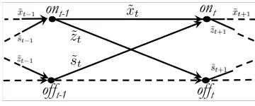
sg,t/zg,t˜ : 1 ifg is turned on / off at timet, 0 otherwise, To see how these variables capture the transition of gener-ator states, we provide an illustration in Fig. 1. In this figure, the on/off status of a generator is denoted with nodes and the feasible state transitions are represented with arcs. Notice that the variables for the decisionremaining off has not been defined and the corresponding arc in Fig.1 is marked with a dashed line. This is because such a transition is completely determined by the values of the other state-transition variables. Indeed, exactly one state transition occurs at each time period, and the corresponding decision variable is set to 1. If none of these variables are set to 1, then the remaining off transition corresponding to the dashed line is said to occur. Following this discussion, it is easy to see that the inequality
˜
sg,t+ ˜xg,t+ ˜zg,t≤1 ∀g∈ G, t∈ T. (15)
is true for any feasible generator schedule formulated with state-transition variables.
on
t-1off
t-1on
toff
t˜ xt
˜ st
[image:5.612.346.526.536.611.2]˜ zt
Fig. 1. Illustration of the state-transition variables.
A deeper look at Fig.1 reveals the network sub-structure embedded in the new formulation. In particular, we observe that a sequence of state transitions of a single generator can be de facto represented by a path on the graph comprising states as nodes and state transitions as arcs. Writing out the flow conservation constraints at the nodes of this graph, we immediately obtain the following state-transition constraints
for the UC problem:
˜
Constraints (16) are the flow conservation constraints at the nodes where the state of the generator is on. At the off
nodes, the flow conservation constraints are the same, therefore omitted. This can be easily verified by assigning the expression
1−sg,t−xg,t˜ −zg,t to the dashed arc in Fig.1. From our perspective, these constraints indicate that if a generator is operational at time t−1 then it must either be turned off or remain on at time t.
The linear mapping(xg,t)→(˜sg,t+˜xg,t)allows us to trans-late any constraint derived for the benchmark formulations into the constraints of our formulation. Although the constraints differ in essence, it is easy to verify that (16) can also be derived from (1a) using the transformation described above.
In a UC problem, the above formulation of the state transitions can potentially lead to significant computational gains, especially when large numbers of state transitions are anticipated. Accordingly, for problems involving longer planning horizons and facing variable demand patterns, one should expect a better performance from this new formulation, compared to contenders that use (x,s,z) variables. While other components of a UC problem can be formulated in alternative ways, the constraints presented in the rest of this section perform well in tandem, and some naturally define the facets of their corresponding polytopes.
a) Formulating production: In our formulation, we opt for the p0
g,t and pg,t¯ variables for formulating production
amounts and reserve requirements. With the state-transition variables, the on/off status of a generator is given by the expression ˜sg,t+ ˜xg,t. Accordingly, theproduction limits for each g∈ G, t∈ T can be given as follows:
¯
pg,t≥p0g,t+Cg¯ (˜sg,t+ ˜xg,t), (17a)
¯
pg,t≤Cg¯ (˜sg,t+ ˜xg,t) + ( ¯
Sg−Cg¯ )˜zg,t+1. (17b)
Constraints (17a) ensure that the maximum possible generation amount at time t (pg,t¯ ) is greater than the actual production amount at the same time period, and constraints (17b) bound
¯
pg,t by the total capacity or the shut down limit of the generator. The minimum production constraints are redundant due to the use of the p0
g,t variables. As is the case in (2),
the variable pg,t¯ must also respect the start up limits, but this restriction is omitted in (17) as it will be implied by the ramping constraints.
The demand constraints of the STF are similar to that of MLR given in (5):
P
g∈G p0g,t+Cg¯ (˜sg,t+ ˜xg,t)
≥dt ∀t∈ T. (18)
Finally, thereserve requirementsare formulated without effort by adopting the constraints in (3).
b) Formulating operational and technological restric-tions: We now formulate the minimum up/downtime and the ramping restrictions. We begin with the former, and translate theminimum up/downtimeinequalities (7) into our formulation as presented below:
Pt−1
i=t−U Tg+1 sg,i˜ ≤xg,t˜ ∀g∈ G, t∈ T, (19a)
Pt
i=t−DTg sg,i˜ ≤1−xg,t˜ −DTg ∀g∈ G, t∈ T. (19b)
Constraint (19a) ensures that if the generator remains on, it could have been turned on at most once in the previousU Tg−
1 time periods. If it does not remain on, then it could not have been turned on in these time periods due to minimum uptime restrictions. Similarly, constraint (19b) ensures that if the generator remains on, it cannot be restarted in the current time period or in the nextDTg time periods due to minimum downtime restrictions. On the other hand, if it does not remain on, it can be turned on at most once in these time periods, due to minimum uptime and downtime restrictions.
To formulate the ramping restrictions, we take advantage of both the state-transition and the production variables, and provide the following ramp up constraints:
¯
pg,t−p0g,t−1≤Sg¯ sg,t˜ +( ¯Rg+Cg¯ )˜xg,t ∀g∈ G, t∈ T. (20a)
The coefficient of the remain-on variable is increased by
¯
Cg because the p0
g,t−1 variable only accounts for the power generation beyond
¯
Cg. When a generator is turned on in period
t, it should have been idle in periodt−1. Thereforep0
g,t−1= 0 and no increment for the ˜sg,t coefficient is necessary. The ramp down constraints are formed in a similar manner and given below.
p0g,t−1−p 0
g,t≤(¯Sg−Cg¯ )˜zg,t+Rg¯ xg,t˜ ∀g∈ G, t∈ T. (20b)
Whenever the generator remains on, the above inequality limits the reduction in the power output such that the ramp down restrictions are obeyed. When the generator is turned off at time t, the inequality reduces to a tight upper bound on the
p0
g,t−1variable. When the reserve requirements are ignored, it can be shown that (20) is equivalent to (10).
c) Linearization of the objective function: For the lin-earization of the start up costs, we opted for the use of the
fg,t variables. Observe that, when turned on, the start up cost of a generator will at least be its warm-start cost, i.e., the start up cost incurred when the generator has not cooled down since the previous operational state. Due to the minimum downtime restriction, this cost is at leastf cDTg
g . Furthermore, it can be
associated with the start up variable and accounted directly in the objective function using the additional termf cDTg
g sg,t.
Therefore, the variablefg,t will now represent the extra cost of turning on a generator which has been idle for some time that is longer than its minimum downtime (DTg). In view of this observation, variablesfg,t must satisfy the followingstart up cost constraints:
fg,t≥(f cτg−f cDTg g)
˜
sg,t−
τ
X
i=DTg
˜
sg,t−i−xg,t˜ −τ
∀g∈ G, t∈ T, andτ ∈ Ig\ {1. . . DTg}
(21)
We note that, in general, the number of constraints to formulate the piecewise-linear cost functions can make mixed-integer programs extremely large. As in MLR, the representa-tion above mitigates this potential issue by eliminating up to |T | ×P
g∈GDTg constraints.
Finally, theproduction costscan be formulated by directly incorporating (14) into our formulation. Similar to MLR, the cost of minimum required production is determined by
¯
d) The state-transition formulation: A summary of the new formulation is provided below:
STF: min X
t∈T
X
g∈G
fg,t+vg,t+ (f c DTg
g +
¯ Cg)sg,t+
¯ Cgx˜g,t
s.t. (3),(16)-(21),(14),(x˜,˜s,˜z)∈ {0,1}3|G||T |,(p,p¯,f,v)≥0
In STF, we do not include constraints (15) as they are implied by minimum downtime constraints (see Appendix A).
III. COMPUTATIONALEXPERIMENTS
Our analysis will focus on two classes of instances. The first stems from the synthetic instances of [13], which are based on [23]. These are single-day instances, involving 24 time periods, and are characterized by increasing numbers of generators. They are known to be challenging for branch-and-bound algorithms, therefore commonly experimented in the literature. Using these instances, we generated two additional data sets. In the first, the numbers of generators are increased tenfold, and in the latter, the time horizon is extended to seven days. Instances with a longer time horizon are more challenging not simply because of the increased dimensions but also due to the daily trends and fluctuations in the demand. The second class of instances are based on the realistic instances obtained through the FERC. Further details can be found in [30]. For both classes of instances, details are given in Appendix B and the references therein.
For dynamic planning models it is well known that the planning horizon can have a significant impact on the de-cisions. The resulting decisions are often myopic, and this phenomenon is commonly referred to as theplanning horizon effect. Such myopic choices can be remedied by choosing to solve longer-horizon models, and only implementing the day-ahead plan. This approach is sometimes also referred to as a receding horizon approach (RHA). In case of the UC model, since a week can be considered as a regeneration point for demands (see [31], [32]), such an RHA is likely to avoid myopic choices. In keeping with this outlook, the choice of a 168 periods reflects the UC problem for the RHA.
In Table I, we present statistics regarding the considered formulations. We observe that the number of binary variables is the same across all formulations. In terms of the numbers of variables, constraints, and nonzero coefficients, STF attains the minimum amounts, leading to compact descriptions of UC problems. We note that the week-long realistic instance contains a significantly larger set of generators compared to other week-long instances that we have experimented with.
All runs were performed on a single thread of a Dell Desktop PC with IntelR CoreTM i7-3770S CPU @ 3.10 GHz, 7.68 GB of RAM, and running Ubuntu Linux 12.04.3 LTS. The formulations were solved with CPLEX 12.5.1. The default parameters ofCPLEXwere preserved, but a time limit of 2 hours is imposed. For instances which could not be solved within this limit, we report the relative optimality gap based on the best available solution and lower bound. It is important to note that the benchmark formulations are true to the mathematical representations provided by the original authors. In making comparisons, certain choices -such as software parameters- are kept the same across all formulations,
TABLE I
FORMULATION STATISTICS(SYNTHETIC INSTANCES WITH|T |= 24
CONTAIN TEN TIMES MORE GENERATORS)
Synthetic Instances (averaged)
|T | Binary / Total Vars. Constraints Nonzeros
OAV 24 77,076 / 179,845 304,789 1,178,779 168 53,953 / 125,892 214,676 868,319
STF 24 77,076 / 179,845 231,313 1,012,799 168 53,953 / 125,892 163,243 748,272
MLR 24 77,076 / 205,537 257,125 1,048,143 168 53,953 / 143,876 181,312 769,461
Realistic Instances
OAV 24 67,608 / 157,753 287,108 1,050,268 168 473,256 / 1,104,265 2,016,548 9,327,706
STF 24 67,608 / 157,753 225,188 925,739
168 473,256 / 1,104,265 1,583,108 8,416,361
MLR 24 67,608 / 180,289 241,532 945,153
168 473,256 / 1,262,017 1,697,516 8,519,871
and no tuning was performed to individually improve their performances.
In Table II, we report the solution times for the synthetic instances, along with the numbers of cuts and nodes generated by the solver. When accompanied with fast solution times, small numbers of cuts could indicate that the instances are amenable to producing integer solutions fast and with little need for tightening. Likewise, small numbers of branch-and-bound nodes (or the lack thereof) imply that the nonconvexity in the instances can be easily tamed. We first make compar-isons on the single-day instances. We observe that STF and MLR perform considerably faster than OAV, especially as the number of generators grow. In terms of solution times, there does not appear to be a significant contender among STF and MLR. However, it is promising to see that the total solution time for all instances is the smallest when STF is used, and the individual times never exceed a minute. Moreover, with STF, all of the instances were solved at the root node, with the minimum number for cutting planes. In contrast, we observe that multiple nodes were explored in a few instances using the benchmark formulations. When we consider week-long instances, we observe an important feature of our formulation. Recall from §II-C that the STF involves an implicit network sub-structure, and it has better potential in capturing the state transitions of the generators between consecutive time periods. Aligned with our expectations in §II-C, we observe that the complexity introduced by a longer time horizon is best tamed with STF. The solution times are significantly better than the benchmark formulations for almost every instance. Furthermore, there are only two instances for which multiple branch-and-bound nodes have been explored. In contrast, the benchmark formulations needed to explore hundreds of nodes to optimize a significant portion of the instances. These results reveal the potential of our formulation to scale up to more realistic instances solved by the power industry.
TABLE II
PERFORMANCE MEASURES OF BRANCH-AND-BOUND FOR SYNTHETIC INSTANCES.
|T |= 24 OAV STF MLR |T |= 168 OAV STF MLR
|G| Cuts/Nodes Time Cuts/Nodes Time Cuts/Nodes Time |G| Cuts/Nodes Time Cuts/Nodes Time Cuts/Nodes Time
280 - / - 2.5 - / - 1.9 - / - 1.1 28 428 / - 3.3 12 / - 3.4 252 / 170 5.8
350 506 / - 5.2 - / - 2.7 - / - 1.6 35 914 / - 6.4 - / - 2.1 865 / - 4.4
440 3,729 / - 11.0 - / - 3.5 - / - 2.2 44 1,188 / - 7.9 - / - 2.8 684 / - 4.9
450 3,867 / - 34.4 218 / - 5.0 1,019 / 100 12.4 45 3,016 / 417 34.3 158 / - 4.7 984 / 413 12.5
490 6,334 / - 29.8 - / - 4.7 63 / - 5.9 49 2,981 / 210 25.1 92 / 75 8.7 517 / 506 21.3
500 9,520 / - 83.5 863 / - 8.5 2,142 / 80 24.7 50 3,191 / 529 61.2 216 / - 6.0 837 / 806 23.1
510 1,850 / - 18.0 - / - 4.3 2 / - 4.6 51 1,263 / - 11.3 18 / - 5.1 105 / - 4.9
510 6,080 / - 23.5 - / - 4.1 - / - 2.8 51 1,550 / - 11.0 - / - 3.1 273 / 185 8.8
520 6,043 / - 26.8 - / - 4.6 1 / - 3.8 52 2,099 / - 14.5 100 / - 4.7 469 / - 6.4
540 7,299 / - 36.0 - / - 4.6 12 / - 4.4 54 2,470 / - 14.7 88 / 63 8.2 373 / 739 21.9
1320 2,676 / - 35.9 - / - 16.1 - / - 9.8 132 1,206 / - 32.9 - / - 11.9 2,159 / - 18.8
1560 12,059 / - 187.2 - / - 23.4 1 / 10 33.4 156 2,781 / - 60.7 51 / - 23.5 285 / 200 39.6
1560 12,737 / - 111.6 - / - 21.6 - / - 19.4 156 3,413 / - 48.3 - / - 15.7 1,994 / 342 52.0
1650 17,249 / - 133.1 - / - 28.6 - / - 23.9 165 6,564 / - 102.8 - / - 21.3 3,306 / 531 89.6
1670 19,588 / - 230.5 - / - 29.6 - / - 27.0 167 8,292 / - 111.1 243 / - 22.1 638 / 1,880 432.2
1720 7,642 / - 81.3 - / - 26.4 - / - 18.9 172 2,705 / - 75.4 310 / - 33.5 2,522 / - 28.2
1820 22,170 / 524 1,069.9 - / - 33.8 753 / 10 61.9 182 7,556 / - 103.6 189 / - 24.6 2,469 / 150 51.8 1820 24,087 / 250 944.3 36 / - 49.1 306 / 485 263.7 182 11,135 / - 171.5 440 / - 25.1 2,935 / 474 101.9
1830 15,978 / - 281.3 - / - 36.7 2 / - 41.8 183 9,038 / - 129.7 285 / - 24.4 1,887 / 577 110.3
1870 24,373 / - 508.8 1,386 / - 58.7 3,636 / - 65.9 187 10,979 / 140 205.9 389 / - 35.4 3,209 / 120 60.4
Total: 203,787 / 774 3,854.3 2,503 / - 367.8 7,937 / 685 629.2 82,769 / 1,296 1,231.8 2,591 / 138 286.3 26,763 / 7,093 1,098.8
made accessible by [30]. The analysis of these instances will provide better intuition on how the new and the benchmark formulations perform in the problems solved in the energy industry. Comparing Table III with Table II, we observe that the differences in the computational performance of the new model and the benchmark formulations are more pronounced. For instance, we observe that OAV hits the time limit on the week-long problem, whereas MLR spends more than 20 minutes to obtain an optimal solution. In comparison, the new model can provide an optimal solution within 12 minutes, achieving a 45% reduction. We conclude our analysis by discussing the percentage of fractional variables in Table III. A small number of fractional variables in the continuous relaxation of the problem could serve as an indication of the tightness of a formulation. Observe that the new formulation provides far larger numbers of integer variables in the linear-programming (LP) relaxations of the problems, confirming the effectiveness of the formulation. The objective value of the LP-relaxation of STF can be 1.4% and 0.2% better than that of OAV and MLR, respectively. More importantly, in the root relaxation (i.e., the starting LP relaxation created within
CPLEX), the percentage of fractional variables shrink even further. Indeed, in the week-long instance, 99.82% of the integer variables are observed to be integral, leading to an almost-integer (lower-bounding) solution.
In order to further assess the behavior of the formulations, we have experimented with modified versions of the original synthetic and realistic instances. In particular, the hourly demand and reserve data are multiplied with (1 +α), where
αis chosen to mimic realistic changes in demand (see [33]). Generator capacities are perturbed with the same coefficient for synthetic instances, however, kept the same for realistic instances, in order to preserve their authenticity. Table IV gives a summary of our analysis. Examining the results for
TABLE III
PERFORMANCE MEASURES OF BRANCH-AND-BOUND AND THE%OF
FRACTIONAL VARIABLES(|G|= 939, RELATIVE OPTIMALITY GAP IS
REPORTED-IN BRACKETS-WHEN THE TIME LIMIT IS HIT)
Branch-and-Bound Frac. Vars. (%)
|T | Cuts/Nodes Time LP/Root Relaxation
OAV 24 4,499 / - 264.1 2.19 / 0.15
168 15,605 / - [0.5%] 1.54 / 0.37
STF 24 478 / 10 53.6 1.09 / 0.13
168 1,940 / - 679.8 0.73 / 0.18
MLR 24 2,914 / - 66.9 2.39 / 0.20
168 11,566 / - 1,243.7 1.76 / 0.29
synthetic instances, we observe that STF is slightly more favored than MLR in the day-long problems, and performs significantly better for the week-long instances. A similar outcome is also observed for the realistic instances, although, for these instances, the performance delivered by STF is consistently better. Notice that the computational gains ob-served for the week-long realistic instances are much larger than the total gains observed for the 20 week-long synthetic instances, indicating the potential of STF for instances with more realistic and diverse problem parameters (e.g., distinct generator capacities, ramping rates, or variable-cost functions with many more pieces).
TABLE IV
SOLUTION TIMES FOR MODIFIED INSTANCES(|G|IS10-FOLD WHEN
|T |= 24FOR SYNTHETIC INSTANCES,AND|G|= 939FOR REALISTIC
INSTANCES).
Synthetic Instances (summed over 20 instances)
|T | α=-5% -2.5% -1% 1% 2.5% 5%
OAV 24 4407.2 4662.3 4363.8 3699.6 4177.9 5343.6 168 1340.2 1154.8 1210.1 1538.2 1484.0 1478.8
STF 24 397.0 367.4 371.8 414.6 491.7 597.5 168 301.2 287.3 300.6 319.8 371.7 348.2
MLR 24 394.3 441.2 367.1 451.1 546.0 579.3 168 730.4 757.3 1111.0 1293.1 916.2 904.0
Realistic Instances
|T | α=-5% -2.5% -1% 1% 2.5% 5%
OAV 24 280.3 328.6 233.8 294.5 167.3 254.7 168 [0.5%] [0.7%] [0.5%] [0.8%] [0.4%] [0.4%]
STF 24 30.4 33.8 35.8 36.0 35.8 33.9 168 835.7 523.2 761.8 712.5 497.2 658.0
MLR 24 58.9 47.7 43.5 49.5 37.7 38.4 168 1417.7 1847.9 1329.7 1336.2 1362.2 1338.1
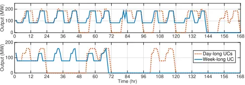
under the commitment decisions of these runs. The same pattern appears for most nonbase-load generators. The day-long problems recommend turning these generators off at the end of each day. In contrast, the week-long problem acts with better foresight and recommends less-frequent state transitions, leading to more stable commitment schedules. More importantly, the week-long problem reports 1.8% lower operational costs.
0 12 24 36 48 60 72 84 96 108 120 132 144 156 168
Output (MW) 0
100 200
Time (hr)
0 12 24 36 48 60 72 84 96 108 120 132 144 156 168
Output (MW)
0 100 200
[image:9.612.53.301.441.527.2]Day-long UCs Week-long UC
Fig. 2. Production patterns of two generators based on the commitment decisions of 7 day-long UC problems, and a week-long problem.
IV. CONCLUSION
In this study, we developed the state-transition formu-lation for the UC problem. Our formuformu-lation replaces the long-established state variables of the UC formulations with state-transition variables. We compare the performance of the new formulation with two benchmark formulations. We observe that the state-transition formulation performs the best
especially for long-horizon instances. The new formulation naturally includes valid inequalities that have been used to strengthen alternative formulations. The induced network sub-structure of the formulation allows the effect of these valid inequalities to propagate throughout the planning horizon.
APPENDIXA
INSIGHTS ON THE POLYHEDRAL STRUCTURE
This appendix summarizes the polyhedral features of our formulation and draws connections with other formulations from the literature. Our discussion will focus on modeling components that involve a single generator, therefore the generator indices are neglected for notational ease. We begin by showing the redundancy of (15) in STF.
Proposition 1. Constraints(15)are implied by the minimum downtime constraints(19b)and the state-transition constraints
(16).
Proof. Consider constraint (19b) for timet+DT−1,
1≥xt˜−1+
t+DT−1 X
i=t−1
˜
si= ˜xt−1+ ˜st−1+
t+DT−1 X
i=t
˜
si [by (16)]
= ˜zt+ ˜xt+ ˜st+
t+DT−1 X
i=t+1
˜
si≥˜zt+ ˜xt+ ˜st.
Remark 1. IfDT= 1, constraints(15)become equivalent to the minimum downtime constraints.
The following definitions and facts will be useful in the remainder of this appendix. We use dim(P) to denote the dimension of a polyhedronP. A facetF ofP has dim(F) =
dim(P)−1. Accordingly, to prove that a constraintπ|x≤π 0 defines a facet ofP, it is sufficient to identify dim(P) affinely-independent points (xi) which satisfy π|xi = π
0, ∀i =
1. . .dim(P). A facet-defining inequality will dominate all other constraints, therefore sought in most polyhedral analyses. For proofs of this type appealing to affine independence for facet-defining inequalities, the reader may refer to [34].
We show that the use of the state-transition decision vari-ables does not affect the polyhedral properties of the original minimum up/downtime constraints (19) of [11], proposed for formulations with (x,s,z) variables. Consider the minimum up/downtime polytope of the STF:
M=
˜s,˜x,˜z∈ {0,1}|T |:
Pt−1
i=t−U T+1 si˜ ≤xt˜ ∀t∈ {U T . . .|T |}, Pt
i=t−DT si˜ ≤1−xt˜−DT ∀t∈ {DT+ 1. . .|T |},
˜
st−1+ ˜xt−1= ˜zt+ ˜xt ∀t∈ {2. . .|T |}.
In the definition above, the history of the generators is ne-glected by removing the corresponding turn on/off constraints defined for periods {1. . . U T −1}, and {1. . . DT}, respec-tively.
Let conv(P)to denote the convex hull of polytopeP.
Proposition 2. The minimum up/downtime constraints (19)
define the facets of the polytope conv(M).
• Consider a set of |T | solutions (˜s,x˜,˜z)i, where i ∈
{1. . .|T |}. This solution has the following structure. The components of the vector s(resp.z) are set to zero with the only exception of the ith component (resp. (i+U T + 1)th
or |T |, whichever is smaller). This element is set to 1. The components of ˜xare set as
˜
xk =
1, i+ 1≤k≤min{i+U T,|T |}
0, otherwise.
• |T | additional solutions(˜s,x˜,˜z)j, j ∈ {1. . .|T |}, which belong to a setJ, are obtained by setting the˜sand˜zvectors to null, while the vector ˜xhas the following components:
˜
xk=
1, k≤j
0, otherwise.
• The last two solutions are (˜s,˜x,z˜) = (0,0,(1,0, . . .0))
and the null solution.
Given the dimension of conv(M), any constraint (19a) is a facet if it has dimension 2× |T |(i.e., if there are2× |T |+ 1
affinely independent solutions which satisfy the inequality as equality). For some t∈ {U T . . .|T |}, consider the set
Ut=
n
˜s,x˜,˜z∈ {0,1}|T |:Pt−1
i=t−U T+1 ˜si= ˜xt o
.
All the solutions listed above belong to the set Ut, with
the exception of |T | −(t+ 1) solutions of set J. In these solutions, the generator is turned off at time t+ 1 or later (i.e., all solutions (˜s,˜x,˜z)j where j > t). For each of these
solutions, turn the generator on at timet−U T+ 1by setting the (t −U T + 1)th component of the vector s to 1, and
setting the first t−U T + 1 components of the vector ˜x to 0. 2× |T |+ 1 affinely independent solutions have thus been generated, proving that Utis a facet of conv(M).
The proof for minimum downtime constraints (19b) is analogous and can be obtained with the same arguments made for constraints (19a).
Next, we show the validity of the ramping inequalities (20), and demonstrate their relation to their counterparts in [13].
Proposition 3. For eacht∈ T, the ramp-up inequality (20a)
is valid and dominates constraint
¯
pt−pt−1≤S¯st˜ + ¯Rxt,˜ (P1a)
which is equivalent to(9a)when the state-transition variables are used.
Proof. It is straightforward to verify the validity of constraints (20a). The inequality limits the increase in production byS¯if the generator has just been turned on (in this case p0
t−1= 0), or by ( ¯R+
¯
C)if it remains on. As also pointed out in§II-A, the ramp-up inequality (P1a) is inactive if the generator has just been turned off; but it can be strengthened by lifting it to the space of zt˜ variables.
¯
pt−hp0t−1+C¯(˜st−1+ ˜xt−1) i
≤S¯st˜ + ¯Rxt˜ −
¯
Czt.˜ (P1b)
The term within brackets ispt−1. To verify that (P1b) is valid, it is sufficient to consider the case where˜zt= 1(the casezt˜ = 0is trivial). As the generator is not operational at time periodt,
¯
ptis 0 and the inequality reduces top0 t−1+
¯
C(˜st−1+ ˜xt−1) =
pt−1 ≥
¯
C, which is the minimum production requirement. Therefore (P1b) is valid and dominates (P1a), which is easy to see as the left-hand side of (P1a) assumes no smaller value than the left-hand side of (P1b). Constraints (20a) can then be obtained from (P1b) using (16):
¯
pt−p0t−1≤S¯˜st+ ¯Rxt˜ −¯Czt˜ +C¯(˜st−1+ ˜xt−1)
= ¯S˜st+ ¯Rxt˜ −
¯
Czt˜ + ¯
C(˜zt+ ˜xt) = ¯S˜st+ ( ¯R+
¯
C)˜xt.
The analysis for the ramp down constraints is provided next.
Proposition 4. For each t ∈ T, the ramp-down inequality
(20b)is valid and dominates the seed inequality pt−1−pt≤
¯
Szt˜+ ¯
Rxt˜, which is equivalent to(9b)when the state-transition variables are are used.
Proof. Consider the seed inequality:
h
p0 t−1+
¯
C(˜st−1+ ˜xt−1) i
−hp0 t+
¯
C(˜st+ ˜xt)i≤
¯
Szt˜ + ¯
Rxt,˜
which can be strengthened by a lifting to the space of˜st,
h
p0t−1+
¯
C(˜st−1+˜xt−1) i
−hp0t+C¯(˜st+˜xt)
i ≤
¯
Szt˜+ ¯
Rxt˜ −
¯
Cst.˜
When ˜st = 1, the power output at time t−1 must be 0, and the first term in brackets disappears. Since xt˜ = ˜zt= 0, the inequality simply reduces to p0
t ≥ 0, which confirms its
validity. By simple algebra, we obtain
p0t−1−p 0
t≤¯Szt˜ + (R¯ +C¯)˜xt−C¯(˜st−1+ ˜xt−1)
= ¯
Szt˜ + ( ¯
R+ ¯
C)˜xt−
¯
C(˜zt+ ˜xt) (P2)
= ( ¯
S−
¯
C)˜zt+ ¯
Rxt˜
where (P2) is achieved using (16).
Using the relations (1a) and (16), it is trivial to verify the following remark.
Remark 2. When the reserve requirements are neglected, the ramping inequalities(20a) and (20b) of the new formulation are equivalent to the facet-defining two-period ramping in-equalities of the base formulation, proposed by [14], i.e., con-straints(10a)and (10b). In contrast, the ramping constraints in MLR are such that the state variables do not explicitly guide the ramping rates of generators.
For our final analysis, we introduce the two-period ramping polytope in our formulation, under the assumption thatU T >
1. For clarity of exposition, we first give the generation and ramping constraints for a givent as follows:
¯
pt≥p0t+C¯(˜st+ ˜xt) (23a)
¯
pt≤S¯st˜ + ¯Cxt˜ + ( ¯
S−C¯)˜zt+1 (23b)
p0t−1−p0t≤(S¯ −C¯)˜zt+R¯xt˜ (23c)
¯
pt−p0t−1≤S¯st˜ + ( ¯R+C¯)˜xt+ (¯S−R¯−C¯)˜zt+1. (23d)
equivalent to thevalid inequality(23) of [13], when written in terms of the state-transition and p0
t−1 variables. We give the two-period ramping polytope below.
R2t =
n
(¯pt, p0t−1, p0t,˜st,xt,˜ zt˜ zt˜+1)∈ <3+× {0,1} 4
:
(23a),(23b),(23c),(23d), st˜ + ˜xt+ ˜zt≤1, zt˜+1 ≤xt˜ o
With respect to the two-period ramping polytope defined in [14], the above definition has some differences. For instance, we consider both the ramp up and ramp down constraints together, which were treated separately in [14]. Furthermore, our polytope is defined in the space of pt¯,p0
t,p0t−1,st˜,xt˜ ,zt˜ andzt˜+1 variables, and considers the reserve requirements.
Proposition 5. Assuming C >¯ R¯ + ¯
R ≥ 2×
¯
R and the generation limit constraints,(23a)and(23b), and the ramping down inequality (23c)and (23d)are facets of conv(R2
t).
Proof. The dimension of conv(R2
t)can at most be 7. In Table
V, we present feasible solutions for this polytope. The first 8 solutions are affinely-independent, thus proving the full dimensionality of conv(R2
t).
TABLE V
SET OF FEASIBLE SOLUTIONS FOR THE TWO-PERIOD RAMPING POLYTOPE.
# p¯t p0t−1 p
0
t ˜st x˜t z˜t z˜t+1 Inactive Cons.
1 0 0 0 0 0 0 0
2 0 0 0 0 0 1 0 (23c)
3 0
¯ S−
¯
C 0 0 0 1 0 (23d)
4 S¯ 0 0 1 0 0 0 (23a)
5 S¯ 0 S¯−
¯
C 1 0 0 0 (23c)
6 C¯ C¯ C¯−
¯
R 0 1 0 0 (23a); (23d)
7
¯ R+
¯
C 2
¯ R
¯
R 0 1 0 0 (23b); (23d)
8
¯ S
¯ S+
¯ R−
¯ C
¯ S−
¯
C 0 1 0 1 (23d)
9 R¯+ ¯ C
¯
R 0 0 1 0 0
Using the solutions displayed in Table V, it is also easy to verify that constraints (23a), (23b), (23c) and (23d) are facet-defining for conv(R2
t). In the last column of Table V, we
report the constraints which are not active in the corresponding solution. To prove that each of the constraints are facet-defining, we modify the coefficients of the solutions in Table V as follows.
• Constraint (23a): change the coefficient of pt¯ from S¯ to
¯
C in Solution 4.
• Constraint (23b): seven solutions out of the eight already satisfy the constraint as equality.
• Constraint (23c): substitute Solution 5 with Solution 9. • Constraint (23d): change the coefficients ofp0
t−1 fromC¯ to C¯ −R¯−
¯
C, from 2 ¯
R to0, and from
¯
S+ ¯
R−
¯
C to
¯
S−R¯−
¯
C in Solutions 6, 7 and 8 respectively.
For each of the constraints, we have provided six affinely independent feasible solutions which satisfy all constraints as equality, thus proving the proposition.
Remark 3. Observe that for everyt∈ T, the inequality(15)
is also facet-defining for conv(R2
t).
APPENDIXB
DETAILS ONDATAGENERATION
A. Synthetic Instances
The instances studied in [13] consider a time horizon of 24 hours, where the hourly demands are given as percentages of the total generation capacity of the system, and the hourly reserve amounts are set to 3% of the resulting demand. To increase the number of generators, we duplicated all generators tenfold, as in [21]. To extend the time horizon, we utilized the demand pattern in our realistic instance (see Appendix B-B). For hour h ∈ {1. . .24} and day d≥ 2, we compute
dh,d/dh,1, where dh,d is the corresponding demand in the realistic instance. These ratios are multiplied with the demand percentages given in [13], and rounded to the nearest integer (see Table VI).
TABLE VI
HOURLY DEMANDS,GIVEN AS PERCENTAGES OF THE TOTAL GENERATION
CAPACITY OF THE SYSTEM(%).
Days Days
Hrs 1 2 3 4 5 6 7 Hrs 1 2 3 4 5 6 7
1 71 68 66 64 63 63 63 13 82 87 87 85 83 87 83
2 65 63 60 58 58 57 58 14 80 85 86 84 82 87 82
3 62 60 58 55 55 55 55 15 79 84 86 84 82 87 82
4 60 59 56 54 54 53 52 16 79 84 87 84 82 88 82
5 58 58 55 52 53 52 50 17 83 88 91 88 86 92 85
6 58 60 57 54 56 54 50 18 91 95 97 94 92 97 91
7 60 66 63 59 62 59 52 19 90 93 93 91 89 92 89
8 64 71 68 65 67 64 56 20 88 90 89 88 87 88 86
9 73 80 76 74 75 73 65 21 85 87 85 84 84 83 82
10 80 86 83 81 81 81 75 22 84 85 83 82 82 81 81
11 82 87 86 84 83 84 79 23 79 79 77 76 76 76 77
12 83 88 87 85 84 87 83 24 74 72 71 70 70 70 72
B. Realistic Instances
The realistic instances of §III are based on the winter test problem, made available by FERC1 and documented in [30]. Here, we only list our assumptions. We set Cg¯ to the seasonal capabilities of the generators, and let Sg¯ = (0.7) ¯Rg,
¯
Sg = (0.7) ¯
Rg.
¯
Cg is either set to the given values, or to min{Sg,¯
¯
Sg}, whichever is the minimum. If no posi-tive value is available, we set them to 1. Likewise, missing
U Tg, DTg are set to 1. We assumed that the minimum up/downtime requirements are not restrictive at t = 0, and generators incur cold start-up cost after 5 time periods. Gener-ators with no cost entries are neglected (104 cases). Finally, we consider the realized demand data2of the PJM region between 01/31/2010 and 01/06/2010, where the former marks the date pertaining to the winter test problem.
REFERENCES
[1] B. Hobbs, M. Rothkopf, R. O’Neill, and H.-P. Chao, Eds., The Next Generation of Electric Power Unit Commitment Models, ser. Inter. Series in Oper. Res. & Mgmt. Sci.. Springer-Verlag, 2001.
1 http://www.ferc.gov/industries/electric/indus-act/market-planning/rto-commit-test.asp
[2] R. P. O’Neill, T. Dautell, and E. Krall, “Recent ISO software enhancements and future software and modeling plans,” FERC, Tech. Rep., 2011. [Online]. Available: http://www.ferc.gov/industries/electric/ indus-act/rto/rto-iso-soft-2011.pdf
[3] A. Turgeon, “Optimal unit commitment,”IEEE Trans. Autom. Control, vol. 23, no. 2, pp. 223–227, 1977.
[4] C. K. Pang, G. B. Sheble, and F. Albuyeh, “Evaluation of dynamic pro-gramming based methods and multiple area representation for thermal unit commitments,”IEEE Trans. Power App. Syst., vol. 100, no. 3, pp. 1212–1218, 1981.
[5] J. Muckstadt and S. A. Koenig, “An application of lagrangian relaxation to scheduling in power-generation systems,”Oper. Res., vol. 25, no. 3, pp. 387–403, 1977.
[6] J. F. Bard, “Short-term scheduling of thermal-electric generators using lagrangian relaxation,”Oper. Res., vol. 36, no. 5, pp. 756–766, 1988. [7] C. Tseng, C. Li, and S. Oren, “Solving the unit commitment problem by
a unit decommitment method,”J. of Opt. Theory, vol. 105, pp. 707–730, 2000.
[8] N. Padhy, “Unit commitment - A bibliographical survey,”IEEE Trans. Power Syst., vol. 19, no. 2, pp. 1196–1205, May 2004.
[9] B. Saravanan, S. Das, S. Sikri, and D. P. Kothari, “A solution to the unit commitment problem - a review,”Frontiers in Energy, vol. 7, pp. 223–236, 2013.
[10] T. Li and M. Shahidehpour, “Price-based unit commitment: a case of lagrangian relaxation versus mixed integer programming,”IEEE Trans. Power Syst., vol. 20, no. 4, pp. 2015–2025, 2005.
[11] D. Rajan and S. Takriti, “Minimum up / down polytopes of the unit commitment problem with start-up costs,” IBM, Tech. Rep., 2005. [12] C. Gentile, G. Morales-Espana, and A. Ramos, “A tight MIP
formu-lation of the unit commitment problem with start-up and shut-down constraints,”EURO Journal on Combinatorial Optimization, 2016. [13] J. Ostrowski, M. F. Anjos, and A. Vannelli, “Tight mixed integer linear
programming formulations for the unit commitment problem,” IEEE Trans. Power Syst., vol. 27, no. 1, pp. 39–46, 2012.
[14] P. Damcı-Kurt, S. K¨uc¸¨ukyavuz, D. Rajan, and A. Atamt¨urk, “A poly-hedral study of production ramping,”Math. Prog., vol. 158, no. 1, pp. 175–205, 2015.
[15] K. Cheung, D. Gade, C. Silva-Monroy, S. M. Ryan, J.-P. Watson, R. J.-B. Wets, and D. L. Woodruff, “Toward scalable stochastic unit commitment,”Energy Systems, pp. 1–22, 2015.
[16] D. Bertsimas, E. Litvinov, X. A. Sun, J. Zhao, and T. Zheng, “Adap-tive robust optimization for the security constrained unit commitment problem,”IEEE Trans. Power Syst., vol. 28, no. 1, pp. 52–63, 2013. [17] A. A. B. Pritsker, L. J. Waiters, and P. M. Wolfe, “Multiproject
scheduling with limited resources: A zero-one programming approach,”
Mgmt. Sci., vol. 16, no. 1, pp. 93–108, 1969.
[18] D. Bertsimas, S. Gupta, and G. Lulli, “Dynamic resource allocation: A flexible and tractable modelling framework,” European Journal of Operational Research, vol. 236, no. 1, pp. 14–26, 2014.
[19] L. L. Garver, “Power generation scheduling by integer programming -development of theory,”Power App. and Syst., Part III, Trans. of the Amer. Inst. of Elect. Eng., vol. 81, no. 3, pp. 730–734, 1962. [20] M. Shahidehpour, H. Yamin, and Z. Li,Market Operations in Electric
Power Systems: Forecasting, Scheduling, and Risk Management. IEEE, Wiley-Interscience, 2002.
[21] G. Morales-Espa˜na, J. M. Latorre, and A. Ramos, “Tight and compact MILP formulation for the thermal unit commitment problem,” IEEE Trans. Power Syst., vol. 28, no. 4, pp. 4897–4908, 2013.
[22] R. Baldick, “The generalized unit commitment problem,”IEEE Trans. Power Syst., vol. 10, no. 1, pp. 465–475, 1995.
[23] M. Carri´on and J. M. Arroyo, “A computationally efficient mixed-integer linear formulation for the thermal unit commitment problem,” IEEE Trans. Power Syst., vol. 21, no. 3, pp. 1371–1378, 2006.
[24] J. M. Arroyo and A. J. Conejo, “Optimal response of a thermal unit to an electricity spot market,”IEEE Trans. Power Syst., vol. 15, no. 3, pp. 1098–1104, 2000.
[25] S. Takriti and J. Birge, “Using integer programming to refine lagrangian-based unit commitment solutions,”IEEE Trans. Power Syst., vol. 15, no. 1, pp. 151–156, 2000.
[26] J. Lee, J. Leung, and F. Margot, “Min-up / min-down polytopes,”
Discrete Optimization, vol. 1, pp. 77–85, 2004.
[27] R. Jiang, Y. Guan, and J. P. Watson, “Cutting planes for the multistage stochastic unit commitment problem,”Math. Prog., vol. 157, no. 1, pp. 121–151, 2016.
[28] K. Pan and Y. Guan, “A polyhedral study of the integrated minimum-up/-down time and ramping polytope,”Optimization Online, 2016.
[29] M. P. Nowak and W. R¨omisch, “Stochastic Lagrangian relaxation applied to power scheduling in a hydro-thermal system under uncertainty,”Ann. Oper. Res., vol. 100, no. 1–4, pp. 251–272, 2000.
[30] E. Krall, M. Higgins, and R. P. O’Neill, “RTO unit commitment test system,” FERC, Tech. Rep., 2012. [Online]. Available: http: //www.ferc.gov/legal/staff-reports/rto-COMMITMENT-TEST.pdf [31] J. Dupaˇcov´a, N. Gr¨owe-Kuska, and W. R¨omisch, “Scenario reduction
in stochastic programming,”Math. Prog., vol. 95, no. 3, pp. 493–511, 2003.
[32] S. Sen, L. Yu, and T. Genc, “A stochastic programming approach to power portfolio optimization,” Oper. Res., vol. 54, no. 1, pp. 55–72, 2006.
[33] New York ISO, “Power trends 2016: The changing energy landscape,” Tech. Rep., 2016. [Online]. Available: http://www.nyiso.com/public/ webdocs/media room/publications presentations/Power Trends/Power Trends/2016-power-trends-FINAL-070516.pdf
[34] G. L. Nemhauser and L. A. Wolsey,Integer programming and combi-natorial optimization. New York: John Wiley and Sons, 1999.
Semih Atakanreceived his B.Sc. degree in man-ufacturing systems engineering, and M.Sc. degree in industrial engineering from Sabancı University, Istanbul, Turkey, in 2010 and 2012, respectively.
He is currently a Ph.D. student at the University of Southern California, Los Angeles, CA. His main research interests are stochastic, convex, and mixed-integer optimization; risk measures; optimization ap-plications, such as power systems planning, disaster management, and scheduling.
Guglielmo Lulli is Senior Lecturer in the Depart-ment of ManageDepart-ment Science at Lancaster Univer-sity. Prior to join Lancaster University, he was Assis-tant Professor at University of Milano-Bicocca. He earned his PhD in Operations Research at University of Rome “La Sapienza” in 2003. During his studies, he visited University of Maryland and University of Arizona, both for one year appointment. He received a Fulbright Fellowship at Massachusetts Institute of Technology, and the 2013 INFORMS TSL Best Published Paper award.
Lulli’s research interests focus on deterministic and stochastic optimization particularly as applied to transportation and logistic operations and energy. He participated in several research projects financed by Italian, European and American agencies.