ISSN Online: 2327-5227 ISSN Print: 2327-5219
DOI: 10.4236/jcc.2017.512003 Oct. 13, 2017 24 Journal of Computer and Communications
A Cloud Computing Fault Detection Method
Based on Deep Learning
Weipeng Gao, Youchan Zhu
Control and Computer Institute, North China Electric Power University, Baoding, China
Abstract
In the cloud computing, in order to provide reliable and continuous service, the need for accurate and timely fault detection is necessary. However, cloud failure data, especially cloud fault feature data acquisition is difficult and the amount of data is too small, with large data training methods to solve a cer-tain degree of difficulty. Therefore, a fault detection method based on depth learning is proposed. An auto-encoder with sparse denoising is used to con-struct a parallel con-structure network. It can automatically learn and extract the fault data characteristics and realize fault detection through deep learning. The experiment shows that this method can detect the cloud computing ab-normality and determine the fault more effectively and accurately than the traditional method in the case of the small amount of cloud fault feature data.
Keywords
Fault Detection, Cloud Computing, Auto-Encoder, Sparse Denoising, Deep Learning
1. Introduction
Cloud computing aims at reducing costs and improving efficiency, serving cus-tomers through resource sharing [1]. Cloud computing, on-demand access, ex-tensive network access, resource pool and other features [2], make its applica-tions more widely. But its breadth and the complexity of the system make the annual rock machine time 5.26 minutes [3], for example: in 2011, the interrupt service Amazon elastic cloud system crash; 2013 Amazon again 45 minutes of downtime. Failures in cloud computing not only cause losses to customers, but also have a significant impact on their reputation and economy [4] [5].
High availability cloud computing needs to be guaranteed by continuously available cloud services, so it is necessary to study fault detection techniques to How to cite this paper: Gao, W.P. and
Zhu, Y.C. (2017) A Cloud Computing Fault Detection Method Based on Deep Learn-ing. Journal of Computer and Communica-tions, 5, 24-34.
https://doi.org/10.4236/jcc.2017.512003
Received: July 20, 2017 Accepted: October 10, 2017 Published: October 13, 2017
Copyright © 2017 by authors and Scientific Research Publishing Inc. This work is licensed under the Creative Commons Attribution International License (CC BY 4.0).
http://creativecommons.org/licenses/by/4.0/
DOI: 10.4236/jcc.2017.512003 25 Journal of Computer and Communications monitor, detect, and maintain continuity of cloud service operations. At present, experts and scholars pay attention to the statistical monitoring method, which is used in the fault detection of cloud computing. Most scholars use Bayesian probabilistic model, decision tree, entropy based and manifold learning algo-rithm for monitoring [6] [7] [8] [9]. Some scholars use cloud adaptive anomaly detection method to detect cloud faults and locate [10] [11] [12] to build high availability cloud computing. These studies are based on historical data analysis, training, and the establishment of a fault model, so as to classify and predict the failure of cloud computing. However, in order to improve the prediction accu-racy of fault classification of cloud computing, cloud computing requires a lot of training to establish a model for fault data, although cloud computing can save the operation data, the active generation means to collect fault data, but these records are relatively few.
In recent years, with the idea of deep learning, depth learning can use a large number of unlabeled data to achieve unsupervised automatic learning [13], through data feature extraction, and then can be used for classification and pre-diction. In 2006, Professor Hinton first proposed the depth of the belief network [14], the depth of its thinking applied to the auto-encoder network to achieve high-dimensional data of low-dimensional features of internal expression [15]. Moreover, with the study of deep learning by many scholars, deep learning has been widely used in various fields such as image recognition [16], Natural Lan-guage Processing [17] and so on. Among them, sparse auto-encoder [18] [19] [20] can use unsupervised automatic learning to abstract the data, and then can be used in classification and prediction, and effectively improve the accuracy. Therefore, a method of fault model detection based on depth learning is pro-posed. First of all, since the sparse auto-encoder automatic learning ability of running state data automatic data feature extraction, during denoising thought, makes the network more robust and stability; then uses the label of data fine-tuning the entire network, makes depth network reached the best effect of classification, and then realizes the cloud computing fault detection.
2. Auto-Encoder
2.1. Depth Auto-Encoder
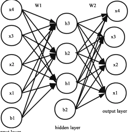
us-DOI: 10.4236/jcc.2017.512003 26 Journal of Computer and Communications ing the model is to obtain data characteristics or nonlinear dimensionality re-duction form of data by obtaining data structure of hidden layer. Its structure is shown in Figure 1.
From left to right, they are input layer, hidden layer and output layer. The mapping between the input layer and the intermediate hidden layer is encoded (edcoder), and the connection weight item W1 between neurons. The mapping between the hidden layer and the output layer is decoded (decoder), and the weight item W2 is connected. The idea of AE is that the input is identical to the output, and the objective function tries to approximate an identity, that is
( )
,W b
h x ≈x. If there are no labeled data sets
{
x x1, , ,2 xn}
, then the costfunc-tion is:
(
)
1 ˆ 2, ; 2
J W b x = x x−
Among them, W is the weight parameter between the encoder neurons, b is the bias value, and the X sample input. ˆx is the actual output. In the encoding phase, the input layer is mapped to the hidden layer via nonlinear functions. The mathematical expressions are as follows:
( )
1 1 11
z W x b a f z
= +
=
Among them, X is the input unlabeled data sample; a is the encoded data after mapping; W is the connection weight between two layers; b is the bias value; f is the encoding activation function; the general is sigmoid function.
[image:3.595.268.484.481.702.2]In the decoding phase, the decoding part is opposite to the encoding, in order to reconstruct the encoded data into the original data, and the expression is as follows:
DOI: 10.4236/jcc.2017.512003 27 Journal of Computer and Communications
( )
2 2 2
2 ˆ
z W a b
x f z
= +
=
Among them, the decoded data is reconstructed; W is the weight between the decoded neurons; b is the bias value; F is the decoding activation function.
2.2. Sparse Auto-Encoder
In the encoder when number of neurons in the input layer is greater than the number of hidden layer neurons, will be forced to automatically learn the cha-racteristics of the hidden layer input data compression feature representation or expression, but when the number of neurons in hidden layer is greater than the input layer number, in order to realize the effect will be better, can through the hidden layer nodes with sparse this restriction, also can obtain the original ex-pression data feature. The sparse auto-encoder is based on the auto-encoder and adds the sparsity restriction to the hidden layer neuron, so that when the num-ber of neurons in the hidden layer is larger, the network can still get better data characteristics.
Sparsity is achieved by whether the neuron is activated. When the neuron's activation function is sigmoid, if the neuron output is close to 1, the neuron is activated; if the output is close to 0, the neuron is suppressed. Therefore, the li-mitation of the sparsity in the network is that neurons are suppressed for most of the time, that is, a small amount of time is activated.
In sparse auto-encoder, in order to make the neurons in the hidden layer most of the time in a suppressed state, can join the sparse penalty factor in the cost function of the model, using the Kullback-Liebler divergence (Kullback-Liebler divergence, KLD) to achieve. KLD is a standard method for measuring the dif-ference between two distributions, so it can be used to measure the change of the sparse penalty factor:
(
)
(
)
2 2
1 1
1 ˆ
|| log 1 log
ˆ 1 ˆ
s s
j
j j j j
KL ρ ρ ρ ρ ρ ρ
ρ ρ = = − = + − −
∑
∑
Among them, ρ is sparse parameter, which indicates the average activity of the preset neuron, which is generally set as 0.05. ρˆj means the average activa-tion degree of neuron j on the training set. The expression for ρˆj is as follows:
( )
( )
1 1
ˆ m i
j j
i a x
m
ρ
=
=
∑
Among them, aj represents the activation of neuronal j, and a xj
( )
represents the overall activation of neurons on the training set X.
Thus, the overall cost function of a sparse encoder can be represented as:
(
)
2 2(
)
sparse
1
1 ˆ ˆ
, ||
2
s
j j
J W b x x λ KL ρ ρ
=
= − +
∑
2.3. Denoising Auto-Encoder
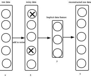
regulariza-DOI: 10.4236/jcc.2017.512003 28 Journal of Computer and Communications tion the auto-encoder The central idea: in the input layer of the original data to add a certain proportion with the statistical properties of the noise, using the self characteristic of encoder to extract useful information of signal extraction, noise removal effective information data in the encoding stage, the realization of orig-inal information reconstruction without any noise in the decoding stage, forcing more robust expression of automatic learning signals from the encoder, such structure is more generalization than other models. Its denoising coding process is shown in Figure 2.
Among them, X is the original signal, and x is the noisy data added to noise. The added noise in raw data is masking noise, Gauss noise, and salt and pepper noise. The masking noise is generally zero in the input data; the Gauss noise is added to the original data to obey the normal distribution of noise; the salt and pepper noise is the input data values randomly set to 0 or 1.
3. Fault Detection Model
[image:5.595.217.533.438.709.2]In the cloud computing failure, the log data collected by the system is easy, and the amount of data is very large, but the fault data is often very small, so you can use a lot of log data, with unsupervised algorithm features encoder auto-matic Learning to extract the inherent characteristics of the data. In this paper, we use the auto-encoder model and the sparse denoising method to form the sparse denoising auto-encoder, and then use the deep learning idea to construct the deep auto-encoder network with sparse denoising to extract the feature data, and finally output classification predictions and realize the detection of cloud computing faults.
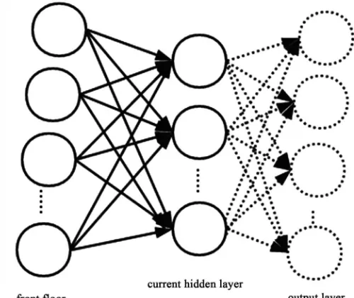
DOI: 10.4236/jcc.2017.512003 29 Journal of Computer and Communications The constructed auto-encoder network fault model consists of three parts: adding noise to the input layer, the depth auto-encoder network in the hidden layer and the classification output layer. The deep auto-encoder network uses the idea of multiple filters in the convolution neural network, the same raw data, extracts a variety of different data features, and uses multiple sparse auto-encoder parallel structures. The fault detection structure is shown in Figure 3.
[image:6.595.216.534.207.712.2] [image:6.595.209.537.217.466.2]In the deep auto-encoder network, the input layer of each sparse auto-encoder adopts the output of the previous layer as input, and the output layer is com-posed of self-built neurons with the same number of neurons. Figure 4 shows.
Figure 3. Fault detection structure.
[image:6.595.247.497.490.700.2]DOI: 10.4236/jcc.2017.512003 30 Journal of Computer and Communications By using the structure of parallel auto-encoder, we can get different fault data features of the same data. The series structure is represented by different fault data features, which is mapped to a higher-level fault feature, and then the data extraction features more abstract and effective.
First, the depth auto-encoder network is initialized. By training, the depth au-to-encoder network is initialized to obtain the locally optimized network weight parameter W and offset b.
Then, fine-tune the entire depth of the auto-encoder network. By using the parameters that have been initialized by training, the tag data is used to fine tune the weight parameters of the network. And finally complete the training of fault classification model.
The entire depth of auto-encoder network fault detection training process is divided into two stages: the network initialization and network fine-tuning. The process is as follows:
1) The first step using a large number of performance data
{ }
xi on the depthof auto-encoder network initialization training
a) Preprocessing performance data
{ }
xi by normalization.b) Set the learning rate
α
, the sparse factor ρ, the denoising ratio ter of the auto-encoder network, and randomly initialize the moment parame-ters W and b.c) According to the number of training and iteration, the forward algorithm is executed and the average activation ρj amount of neurons is calculated.
d) Reverse the algorithm, update the network parameters W and b.
2) The second step through the label performance data
{
x y yi, i}
, ∈{
1,2, , k}
and fault data on the depth of auto-encoder network fine-tuning training a) Initialize the network parameters using the updated network parameters W and b in step (1).
b) Normalized tagged data set
{
x y yi, i}
, ∈{
1,2, , k}
.c) to carry forward the algorithm, calculate the cost function of the network. d) to reverse the algorithm, iterative update network parameters W and b, the weight of the fine-tuning.
At the beginning of the initialization of the depth of the network, when the output classification layer does not have the conditions to build sparse au-to-encoder, the final output layer does not need to initialize, directly use the BP algorithm to fine-tune to the optimal. Finally use the test set to test the entire network.
4. Test Results and Analysis
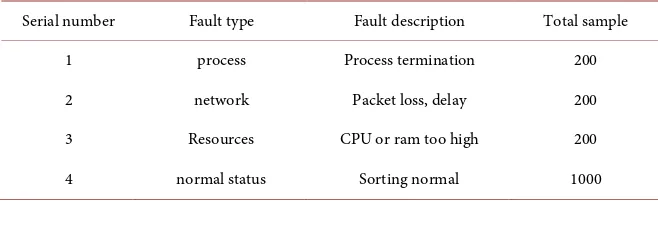
DOI: 10.4236/jcc.2017.512003 31 Journal of Computer and Communications usage, I/O, and data exchange, through third-party testing tools Sysstat. The Hadoop platform uses the built-in tersort test program for sorting testing. In order to verify, through the manual injection of the failure of the way, including the normal state, including the collection of four states to experiment, the status samples are shown in Table 1.
In the experiment randomly selected 3/4 as a training sample, 1/4 as the number of test samples. In the experiment, the network adopts the untagged da-ta preprocessing to initialize the deep auto-encoder network part, using the label data instead. At the correct rate, true positive rate (TPP) and subsequence false positive rate (SFPR) are used:
The number of abnormal samples detected TPR
Abnormal sample size
=
The number of samples is normally detected incorrectly SFPR
Abnormal sample size
=
In this fault model, because of the idea of adding sparse denoising, it will cer-tainly affect the performance of the whole network. Therefore, in comparison, we add auto-encoder network, sparse auto-encoder network, and sparse denois-ing auto-encoder network. The last layer is the fault output classification layer, and the proportion of noise added is set to 1% according to the overall perfor-mance considerations. Therefore, the final experimental results in the experi-ment are shown in Table 2.
It can be seen from Table 2 that adding sparse auto-encoder has better accu-racy than auto-encoder, indicating that sparsely auto-encoder have the ability to better extract intrinsic features of data, which in turn increases the ability to classify faults; The results show that the accuracy of the detection accuracy is not decreased when the denoising is applied, and there is a certain anti-jamming ca-pability of noise data.
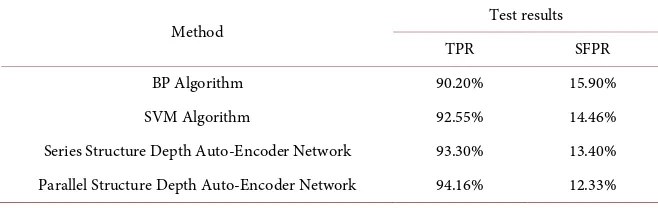
And then through the traditional algorithm such as BP algorithm, SVM algo-rithm and stack-type structure of the depth of auto-encoder network. The sparse de-noising auto-encoder network adopts 10-layer structure. The BP algorithm adopts the 5-layer structure of the same number of hidden layer neurons in the auto-encoder network. The experimental results are shown in Table 3.
[image:8.595.209.538.618.732.2]As can be seen from Table 3.
Table 1. Status samples.
Serial number Fault type Fault description Total sample
1 process Process termination 200
2 network Packet loss, delay 200
3 Resources CPU or ram too high 200
DOI: 10.4236/jcc.2017.512003 32 Journal of Computer and Communications Table 2. Test results table.
[image:9.595.209.538.208.312.2]Method Test results TPR SFPR Auto-Encoder Network 92.18% 15.87% Sparse Auto-Encoder Network 94.15% 13.28% Sparse De-noising Auto-Encoder Network 94.16% 12.33%
Table 3. Test results table.
Method Test results TPR SFPR BP Algorithm 90.20% 15.90% SVM Algorithm 92.55% 14.46% Series Structure Depth Auto-Encoder Network 93.30% 13.40% Parallel Structure Depth Auto-Encoder Network 94.16% 12.33%
Since the series structure depth encoding network compared to the BP algo-rithm and the SVM algoalgo-rithm has better accuracy, but compared with parallel structure since the depth encoding network, accuracy slightly worse, indicates that in the parallel structure of the depth of auto-encoder network for the series data extraction feature is superior to simple, accurate . So the parallel structure of the depth of auto-encoder network fault detection capability is more accurate.
Finally, according to the experimental result, the proposed depth auto-encoder network fault detection method in dealing with cloud fault feature, has obvious advantages, detection method has a certain degree of accuracy, and can be ap-plied to cloud computing system security and reliability assurance system.
5. Conclusion
In order to ensure the stability and reliability of cloud computing system, a deep auto-encoder network fault detection method is proposed. The method firstly extracts the feature data from the depth auto-encoder network with sparse de-noising idea, and then uses the neural network classification output, fault detec-tion. Experimental results show that the deep auto-encoder network with sparse denoising idea is more accurate for cloud fault detection. Compared with single support vector machines and BP networks, it has more effective fault detection capability.
References
[1] Li, L.Y. (2013) Cloud Computing and Practical Technology. China University of Drop Press, Beijing, 23-26.
DOI: 10.4236/jcc.2017.512003 33 Journal of Computer and Communications [3] Chen, H.P., Xia, G.B. and Chen, R. (2013) The Platform’s Research and Prospect of High Performance Computing Technology with Cloud Computing. High Scalability and High Dependability, 3, 29-30.
[4] Patterson, D.A. (2002) A Simple Way to Estimate the Cost of Downtime. Proceed-ings of the 16th USENIX Conference on System Administration, Philadelphia, USA, 185-188.
[5] Bouchenak, S. and Chockler, G. (2013) Verifying Cloud Services: Present and Fu-ture. ACM SIGOPS Operating Systems Review, 47, 6-19.
https://doi.org/10.1145/2506164.2506167
[6] Guan, Q., Zhang, Z.M. and Fu, S. (2012) Ensemble of Bayesian Predictors Arid De-cision Trees for Proactive Failure Management in Cloud Computing Systems. Jour-nal of Communications (JCM), 7, 52-61.
[7] Modi, C.N., Patel, D.R., Patel, A., et al. (2012) Bayesian Classifier and Snort Based Network Intrusion Detection System in Cloud Computing. Computing Communi-cation & Networking Technologies (ICCCNT), Coimbatore, USA, 1-7.
[8] Wang, C.W. and Talwar, V. (2010) Online Detection of Utility Cloud Anomalies Using Metric Distributions. Network Operations and Management Symposium (NOMS), Osaka, USA, 96-103.
[9] Chen, D.W., Hou, N. and Sun, Y.Z. (2010) A Calculation Model for Intrusion De-tection of Computer Science Improved Manifold Learning Method Based on the Cloud. Computer Science, 37, 59-62.
[10] Pannu, H.S., Liu, J.G. and Fu, S. (2012) A Self-Evolving Anomaly Detection Framework for Developing Highly Dependable Utility Clouds. Global Communica-tion Conference (GLOBHCOM), Anaheim, CA, 3-7 December 2012, 1605-1610. https://doi.org/10.1109/GLOCOM.2012.6503343
[11] Xia, M.N., Gong, D. and Xiao, J. (2014) An Adaptive Fault Detection Method for Reliable Cloud Computing. Computer Application Research, 31, 426-430.
[12] Wang, T., Gu, Z., Zhang, W., Xu, J., Wei, J. and Zhong, H. (2016) A Fault Detection Method for Cloud Computing Systems Based on Adaptive Monitoring. Proceedings of the Chinese Society of Computers, 1-16.
[13] Cheriyadat, A.M. (2014) Unsupervised Feature Learning for Aerial Scene Classifica-tion. IEEE Transactions on Geoscience & Remote Sensing, 2, 439-451.
https://doi.org/10.1109/TGRS.2013.2241444
[14] Hinton, G.E., Osindero, S. and Teh, Y.W. (2006) A Fast Learning Algorithm for Deep Belief Nets. Neural Computation, 18, 1527-1554.
https://doi.org/10.1162/neco.2006.18.7.1527
[15] Hinton, G.E. and Alakhutdinov, R.R. (2006) Reducing the Dimensionality of Data with Neural Networks. Science, 13, 504-507.
[16] Krizhevsky, A., Sutskever, I. and Hinton, G.E. (2012) Image Net Classification with Deep Convolutional Neural Networks. Advances in Neural Information Processing Systems, 5, 1106-1114.
[17] Hinton, G., Eng, L.U.D., et al. (2012) Deep Neural Networks for Acoustic Modeling in Speech Recognition: The Shared Views of Four Research Groups. IEEE Signal Processing Magazine, 9, 82-97.
[18] Wright, J., Ma, Y., Mairal, J., et al. (2010) Sparse Representation for Computer Vi-sion and Pattern Recognition. Proceedings of IEEE, 8, 1031-1044.
Sys-DOI: 10.4236/jcc.2017.512003 34 Journal of Computer and Communications tems, Vancouver, 1185-1192.
[20] Boureau, Y.L., Ach, F., Ecun, Y., et al. (2010) Learning Mid-Level Features for Rec-ognition. IEEE Conference on Computer Vision and Patten Recognition, San Fran-cisco, 13-18 June 2010, 2559-2566.