Patterns of synchrony in coupled cell networks with multiple arrows

This paper is made available online in accordance with

publisher policies. Please scroll down to view the document

itself. Please refer to the repository record for this item and our

policy information available from the repository home page for

further information.

To see the final version of this paper please visit the publisher’s website.

access to the published version may require a subscription.

Author(s): Martin Golubitsky, Ian Stewart and Andrei Torok

Article Title: Patterns of Synchrony in Coupled Cell Networks with

Multiple Arrows

Year of publication:2005

Vol. 4, No. 1, pp. 78–100

Patterns of Synchrony in

Coupled Cell Networks with Multiple Arrows∗

Martin Golubitsky†, Ian Stewart‡, and _{Andrei T¨or¨ok}†

Abstract. A coupled cell system is a network of dynamical systems, or “cells,” coupled together. The archi-tecture of a coupled cell network is a graph that indicates how cells are coupled and which cells are equivalent. Stewart, Golubitsky, and Pivato presented a framework for coupled cell systems that permits a classification of robust synchrony in terms of network architecture. They also studied the existence of other robust dynamical patterns using a concept of quotient network. There are two difficulties with their approach. First, there are examples of networks with robust patterns of synchrony that are not included in their class of networks; and second, vector fields on the quotient do not in general lift to vector fields on the original network, thus complicating genericity arguments. We enlarge the class of coupled systems under consideration by allowing two cells to be coupled in more than one way, and we show that this approach resolves both difficulties. The theory that we develop, the “multiarrow formalism,” parallels that of Stewart, Golubitsky, and Pivato. In addition, we prove that the pattern of synchrony generated by a hyperbolic equilibrium isrigid(the pattern does not change under small admissible perturbations) if and only if the pattern corresponds to a balanced equivalence relation. Finally, we use quotient networks to discuss Hopf bifurcation in homogeneous cell systems with two-color balanced equivalence relations.

Key words. coupled systems, synchrony, bifurcation

AMS subject classifications. 34C15, 34C23, 34A34, 37C99, 37G15

DOI. 10.1137/040612634

1. Introduction. Stewart, Golubitsky, and Pivato [10] formalize the definition of a coupled cell system in terms of the symmetry groupoid of an associated coupled cell network and prove three general theorems about such networks. First, a set of cells can be robustly synchronous if and only if the cells are in the same equivalence class of some balanced equivalence relation. Second, every balanced relation leads to a new coupled cell network, called a quotient network, that is formed by identifying equivalent cells. Third, the restriction of a coupled cell system to a synchrony subspace (or polydiagonal) is a coupled cell system associated to the quotient network. The approach in [10] has two difficulties:

(1) Not every coupled cell system of ODEs corresponding to the quotient network is the restriction of a coupled cell system corresponding to the original network. This fact makes it difficult to prove genericity statements about dynamics in the original network based only on genericity statements about dynamics of the quotient network. (Dias and

∗_{Received by the editors October 21, 2003; accepted for publication (in revised form) by G. Kriegsmann July 30,}

2004; published electronically February 22, 2005. This work was supported in part by NSF grant DMS-0244529 and ARP grant 003652-0032-2001.

http://www.siam.org/journals/siads/4-1/61263.html

†_{Department of Mathematics, University of Houston, Houston, TX 77204-3008 ([email protected],}

[email protected]).

‡_{Mathematics Institute, University of Warwick, Coventry CV4 7AL, UK ([email protected]). The work}

of this author was supported in part by a grant from EPSRC.

Stewart [3] obtain necessary and sufficient conditions, on a network with a balanced relation, for every quotient system to be a restriction of a cell system corresponding to the original network.)

(2) Reasonable networks that are not included in the theory developed in [10] can exhibit patterns of robust synchrony. Examples are linear chains with Neumann boundary conditions considered in Epstein and Golubitsky [5] and square arrays of cells with Neumann boundary conditions considered in Gillis and Golubitsky [6].

In this paper we show that both of these difficulties can be resolved if the class of coupled cell networks is enlarged to permit multiple couplings between cells and self-coupling. We call this the multiarrow formalism for coupled cell networks. Although the abstract definition of this enlarged class of coupled cell networks is more complicated than the more restrictive definition in [10], the multiarrow formalism has the side benefit that quotient systems are more easily defined in the enlarged class and have more convenient properties.

We first motivate the generalization by considering two examples in the important case of a homogeneous network, which we now define. A cell is a system of ODEs, and a coupled cell system is a collection of N cells with couplings. As discussed in [10], a class of coupled cell systems is defined by a coupled cell network, which is a (directed, labeled) graph that specifies, among other information, which cells are coupled to which. Two cells of the network areinput isomorphic(see [10]) if the dynamics of the cells are specified by the same differential equations, up to a permutation of the variables. More precisely, if cells 1 and 2 with internal state variables x₁, x₂ ∈Rk are input isomorphic, then the relevant components of the system of ODEs take the form

˙

x₁ = f(x₁, y₁, . . . , y_l), ˙

x₂ = f(x₂, z₁, . . . , z_l), (1.1)

where theyj (resp.,zj) are internal state variables of the cells connected to cell 1 (resp., cell 2).

In particular, the two cells receive inputs from the same number lof cells, the input variables are of the same type y_j, z_j ∈Rkj_{, and the dependence of the corresponding components of ˙x} is specified using the same function f of the relevant internal variables and input variables. The phase space of the coupled cell system is

P ={x= (x₁, . . . , xn)∈Rk1 × · · · ×RkN}.

We call a coupled cell network homogeneous if all cells are input isomorphic (in which case k₁ =· · ·=kN). Homogeneous coupled cell systems are determined by a single function

f, as illustrated in (1.1). For the remainder of this introduction we focus on homogeneous coupled cell networks.

We can visualize an equivalence relationon cells by coloring all equivalent cells with the same color. This equivalence relation is balanced(in the homogeneous case with one kind of coupling) if the sets of colors of input cells for two equivalent cells consist of the same colors with the same multiplicities. Theorem 6.5 of [10] states that the subspace

∆={x∈P :x_i =x_j if i j}

is flow-invariant for allf if and only ifis balanced. A solution in ∆ issynchronousin the

robustin the sense that it holds for any choice off. We call ∆thepolydiagonalorsynchrony subspace corresponding to.

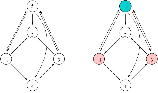
Quotients lead to multiple arrows. We describe circumstances in which multiple arrows are natural and useful. Consider the homogeneous five-cell coupled cell network pictured in Figure 1 (left). A balanced coloring of this network is given in the right panel of that figure.

1

2

3

4 5

1

2

3

4 5

Figure 1. (Left) Homogeneous five-cell network. (Right) Balanced coloring of the network.

The differential equations corresponding to this five-cell network have the form

˙

x₁ = f(x₁, x₂, x₅),

˙

x₂ = f(x₂, x₃, x₅),

˙

x₃ = f(x₃, x₄, x₅),

˙

x₄ = f(x₄, x₁, x₅),

˙

x₅ = f(x₅, x₁, x₃),

wheref(a, b, c) =f(a, c, b) since all couplings are assumed to be identical. It is straightforward to check that the subspace ∆ defined byx₁=x₃ andx₂ =x₄ is flow-invariant. The restricted system on ∆ has the form

˙

x₁ = f(x₁, x₂, x₅),

˙

x₂ = f(x₂, x₁, x₅),

˙

x₅ = f(x₅, x₁, x₁).

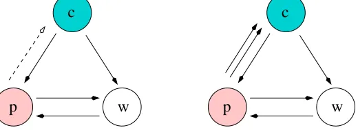
The quotient cell construction in [10] leads to the coupled cell network of Figure 2(left). The coupled cell system corresponding to that quotient network, which is not homogeneous, has the form

˙

w = f(w, p, c), ˙

p = f(p, w, c), ˙

c = g(c, p).

where f(a, b, c) = f(a, c, b). In this paper we remove such conditions from consideration by allowing multiple couplings between cells. With multiple couplings, the quotient network is the homogeneous one of Figure 2(right). Quotient coupled cell systems for the new quotient have the form

˙

w = f(w, p, c), ˙

p = f(p, w, c), ˙

c = f(c, p, p),

and each of these systems is the restriction to ∆ of a five-cell system. Homogeneous three-cell networks with each cell having at most two input arrows are classified in [9]. See Figure 8; there are 34 such networks.

p w

c

p w

c

Figure 2. (Left) Three-cell quotient from [10]of five-cell network in Figure 1(right). (Right) Three-cell quotient using multiarrows.

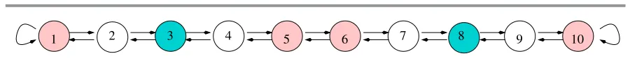
Neumann boundary conditions lead to self-coupling. We now provide a reason for per-mitting self-coupling. Epstein and Golubitsky [5] consider patterns of synchrony in N-cell bidirectional linear arrays with Neumann boundary conditions. The systems of ODEs have the form

˙

x₁ = f(x₁, x₁, x₂), ˙

xj = f(xj, xj−1, xj+1), 1< j < N,

˙

x_N = f(x_N, x_N−1, x_N),

where f(a, b, c) = f(a, c, b). When self-coupling of a cell to itself is allowed, the network architecture is the one pictured in Figure 3.

1 2

.

.

.

Figure 3. Linear array network.

1 2 3 4 5 6 7 8 9 10

Figure 4. Linear array network of ten cells with a three-color balanced relation.

Structure of the paper. The paper is structured as follows. The enlarged class of “mul-tiarrow” coupled cell networks, which permits multiple arrows and self-coupling, is defined in section2. The associated admissible vector fields are constructed in section3. In that section we also show that distinct networks in the enlarged class can correspond to the same space of admissible vector fields. We call two such networksODE-equivalent. This (undesired) feature is not present in the class of networks considered in [10]. The connection between balanced equivalence relations and robust polysynchrony is discussed in section 4. In this section we prove Theorem4.3, which states that flow-invariant subspaces correspond to balanced equiv-alence relations in the multiarrow formalism. Quotient networks are defined in the context of multiple arrows and self-coupling in section 5. In Theorem 5.2 we show that all admissible vector fields on a quotient network lift to admissible vector fields on the original network, a property that fails for the quotients defined in [10].

Some examples of coupled cell networks with self-coupling and multiple arrows are dis-cussed in section 6. The important special case of identical-edge homogeneous networks (ho-mogeneous networks in which all coupling arrows are equivalent) is considered in section 8. Proposition8.2states that every homogeneous network with multiarrows and/or self-coupling is a quotient of a homogeneous network with neither multiarrows nor self-coupling. In sym-metric networks, Hopf bifurcation typically leads to periodic states in which some cells have identical waveforms (hence identical amplitudes) except for a well-defined phase shift. In sec-tion 9 we show that in identical-edge homogeneous networks, Hopf bifurcation can lead to periodic states with well-defined approximatephase shifts and differentamplitudes.

As noted, Theorem4.3states that flow-invariant subspaces can be identified with balanced equivalence relations. Theorem 7.6 strengthens this result by showing that if a hyperbolic equilibrium has a pattern of synchrony that does not change under small admissible pertur-bations, then the subspace corresponding to this pattern of synchrony is flow-invariant and hence corresponds to a balanced equivalence relation.

The proofs of several of the main theorems in this paper (particularly Theorems 4.3and

5.2(a)) are straightforward adaptations of corresponding results in [10] to the enlarged cat-egory of networks considered here. The general results that go beyond those in [10] are the lifting of quotient vector fields (Theorem5.2(b)) and the result that rigid hyperbolic equilibria correspond to balanced equivalence relations (Theorem 7.6).

2. Coupled cell networks. We begin by formally defining a class of coupled cell networks that permits multiple arrows and self-couplings.

Definition 2.1. In the multiarrow formalism, a coupled cell network G consists of the fol-lowing:

(a) A finite set C={1, . . . , N} of nodes or cells.

(c) A finite set E of edges or arrows.

(d) An equivalence relation ∼E on edges in E. Thetype or coupling label of edge eis the

∼E-equivalence class [e]E of e.

(e) Two maps H:E → C and T :E → C. For e∈ E we callH(e) the head of eand T(e) the tailof e.

We also require a consistency condition:

(f) Equivalent arrows have equivalent tails and heads. That is, if e₁, e₂∈ E and e₁ ∼E e₂, then

H(e₁)∼C H(e₂), T(e₁)∼C T(e₂).

Observe that self-coupling is permitted (that is, we allow H(e) = T(e)) and multiple arrows are permitted (it is possible to have H(e₁) =H(e₂) andT(e₁) =T(e₂) for e₁ =e₂).

Associated with each cell c ∈ C is an important set of edges, namely, those that will be interpreted as representing couplings into cell c.

Definition 2.2. Let c∈ C. Then theinput set of c is

I(c) ={e∈ E :H(e) =c}.

(2.1)

An element of I(c) is called an input edge or input arrow of c. The following concept is fundamental.

Definition 2.3. The relation ∼I of input equivalence on C is defined byc∼I d if and only if there exists an arrow-type preserving bijection

β:I(c)→I(d).

(2.2)

That is, for every input arrow i∈I(c)

i∼E β(i).

(2.3)

Any such bijection β is called an input isomorphismfrom cell c to cell d. The set B(c, d) denotes the collection of all input isomorphisms from cell c to cell d. The set

BG =

c,d∈C

B(c, d)

(2.4)

is a groupoid (Brandt[1], Brown [2], Higgins[8]), which is an algebraic structure rather like a group, except that the product of two elements is not always defined. We call B_G thegroupoid of the network. Note that the union in(2.4) is disjoint and thatB(c, c)is a permutation group acting on the input set I(c).

The definitions of input equivalence, input isomorphism, and groupoid of the network are direct generalizations to the multiarrow context of Definitions 3.2 and 3.5 in [10]. By the consistency condition (f) of Definition 2.1, c ∼_I d implies c ∼_C d, but the converse fails in general.

(b) The reason for introducing an explicit set I(c) of input arrows is to provide a well-defined set for the input isomorphismβ in (2.2) to act on. Otherwise we must consider “sets” in which elements may occur more than once. This is the main novelty in Definition 2.3 compared to that in [10].

There does exist a standard theory of such “sets,” which are called multisets. See Wild-berger [12]. The multiarrow formalism could also be set up in multiset language.

Definition 2.5.A homogeneous network is a coupled cell network such thatB(c, d)=∅for every pair of cells c, d.

3. Vector fields on a coupled cell network. We now define the class F_GP of admissible vector fields corresponding to a given coupled cell networkG. This class consists of all vector fields that are “compatible” with the labeled graph structure or, equivalently, are “symmetric” under the groupoidB_G. It also depends on a choice of “total phase space”P, which we assume is fixed throughout the subsequent discussion.

For each cell in C define a cell phase space P_c. This must be a smooth manifold of dimension ≥ 1, which for simplicity we assume is a nonzero finite-dimensional real vector space. We require

c∼_C d =⇒ P_c=P_d,

and we employ the same coordinate systems on P_c and P_d. Only these identifications of cell phase spaces are canonical; that is, the relation c ∼C d implies that cells c and d have the

same phase space but not that they have isomorphic (conjugate) dynamics. Define the correspondingtotal phase spaceto be

P =

c∈C

P_c

and employ the coordinate system

x= (xc)c∈C

on P.

More generally, suppose that D= (d₁, . . . , d_s) is any finite ordered subset of scells in C. In particular, the same cell can appear more than once in D. Define

P_D=P_d1 × · · · ×P_ds.

Further, write

x_D = (x_d1, . . . , x_ds),

where x_dj ∈P_dj.

For a given cell c theinternal phase spaceisP_c and thecoupling phase spaceis

whereT(I(c)) denotes the ordered set of cells (T(i₁), . . . ,T(i_s)) as the arrowsi_k run through

I(c). Suppose c, d∈ C andc∼Id. For anyβ ∈B(c, d), define thepullback map

β∗ :P_T(I(d))→P_T(I(c))

by

(β∗(z))_T(i)=z_T(β(i))

(3.1)

for all i∈ I(c) and z ∈ P_T(I(d)). We use pullback maps to relate different components of a vector field associated with a given coupled cell network. Specifically, the class of vector fields that is encoded by a coupled cell network is given in Definition 3.1.

Definition 3.1. A vector fieldf :P →P isBG-equivariantor G-admissibleif the following hold:

(a) For allc∈ C the componentf_c(x)depends only on the internal phase space variablesx_c

and the coupling phase space variablesx_T(I(c)); that is, there existsfˆc :Pc×PT(I(c))→

Pc such that

fc(x) = ˆfc(xc, xT(I(c))).

(3.2)

(b) For all c, d∈ C andβ ∈B(c, d)

ˆ

f_d(x_d, x_T(I(d))) = ˆf_c(x_d, β∗(x_T(I(d)))) (3.3)

for all x∈P.

Observe that self-coupling is allowed (that is,P_c can be one of the factors inP_T(I(c))) and multiple arrows between two cells are allowed (since the tail of two arrows terminating inI(c) can be the same cell). However, when repetition occurs, the repeated coordinates are always identical.

It follows thatf is determined if we specify one mapping for each input equivalence class of cells. Indeed, each admissible vector field on a homogeneous cell system is uniquely determined by a single mappingf_c at some nodec. In general, each component f_c off is invariant under the vertex groupB(c, c). Indeed, every such invariant function determines a unique admissible vector field.

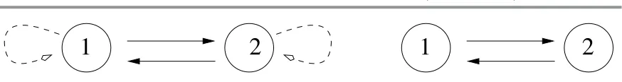
ODE-equivalent networks. In the enlarged class of coupled cell networks, it is possible for two different coupled cell systems G₁ and G₂ to generate the same space of admissible vector fields. For instance, consider the two two-cell systems in Figure 5. Their corresponding systems of admissible vector fields are

˙

x₁ = g(x₁, x₁, x₂), ˙

x₂ = g(x₂, x₂, x₁) and ˙

x₁ = f(x₁, x₂), ˙

x₂ = f(x₂, x₁).

1

2

1

2

Figure 5. Two ODE-equivalent networks.

4. Balanced equivalence relations. We now extend the key concept of a balanced equiv-alence relation to the multiarrow formalism and generalize its properties.

Definition 4.1.An equivalence relation onC is balancedif for everyc, d∈ C withc d, there exists an input isomorphism β ∈B(c, d) such that T(i)T(β(i))for all i∈I(c).

In particular,B(c, d)=∅implies c∼I d. Hence, balanced equivalence relations refine∼I. In the important special case where all pairs of arrows connecting the same two cells are ∼E-equivalent, there is a graphical way to test whether a given equivalence relation

is balanced. Color the cells in a network so that two cells have the same color precisely when they are in the same -equivalence class. Then is balanced if and only if every pair of identically colored cells admits a color-preserving input isomorphism (more precisely, an input isomorphismβ whereT(i) andT(β(i)) have the same color). For example, consider the balanced relation in the network in Figure 1 (right).

Choose a total phase spaceP, and letbe an equivalence relation onC. We assume that is a refinement of ∼_C; that is, if c d, then c and d have the same cell labels. It follows that the polydiagonal subspace

∆={x∈P :xc =xdwheneverc d ∀c, d∈ C}

is well defined, sincex_c andx_dlie in the same spaceP_c =P_d. The polydiagonal ∆is a linear subspace ofP.

Definition 4.2. Letbe an equivalence relation onC. Thenisrobustly polysynchronous if ∆ is invariant under every vector field f ∈ F_GP. That is,

f(∆)⊆∆

for all f ∈ F_GP. Equivalently, if x(t) is a trajectory of any f ∈ F_GP, with initial condition

x(0)∈∆, then x(t)∈∆ for allt∈R.

We now generalize Theorem 6.5 of [10] to the multiarrow formalism.

Theorem 4.3. Let be an equivalence relation on a coupled cell network. Then is robustly polysynchronous if and only if is balanced.

Proof. The proof is essentially the same as that of Theorem 6.5 of [10]. The main points are that it is easy to check directly thatbeing balanced is sufficient for ∆ to be robustly polysynchronous, while necessity can be established by considering admissible linear vector fields. We take these points in turn.

First, suppose thatis balanced, and letf ∈ F_GP. Suppose thatc d. By Definition4.1 the set B(c, d) is nonempty, so there exists β∈B(c, d). We haveβ(c) =d.

We know that for all c ∈ C the component fc(x) is symmetric under all permutations of

the input set I(c) that preserve-equivalence classes. Therefore, for any x∈∆,

because β preserves the -equivalence classes. Therefore,f leaves ∆ invariant. For the converse, suppose that ∆is invariant under allf ∈ FP

G. Then, in particular, ∆

is invariant under all linear f ∈ F_GP. Letc=d∈ C withc d. We first show that c∼I d. If not, we can define an admissible linear vector fieldf such thatf_c = 0, f_d= 0. This contradicts invariance of ∆. Therefore, c d implies thatc, dare input-equivalent as claimed.

Next, we construct a class of admissible linear vector fields as follows. For each pair of

∼C-equivalence classes of cells ([c],[d]) choose representatives c, d ∈ C. Choose some linear map

λ_dc:P_d→P_c.

Ifc ∼C candd ∼C d, use the canonical identifications ofP_c withP_c and P_d withP_dto pull back λdc to a linear map

λdc :Pd →Pc.

That is, we ensure that λdc remains “the same” map when cells are replaced by canonically

identified cells.

Now choose a transversal R to the set of ∼I-equivalence classes. That is, arrange for R to contain precisely one member of each ∼I-equivalence class. For each t∈ R define

Λ_t(x) =

i∈I(t)

λ_T(i)t(x_T(i)).

If i, j∈I(t) and i∼E j, impose the extra condition

λ_T(i)t=λ_T(j)t,

(4.1)

where we canonically identify P_T(i) with P_T(j). Condition (4.1) ensures that Λt is B(t, t

)-invariant.

Any c ∈ C is ∼I-equivalent to precisely one t(c) ∈ R. Let β ∈ B(t(c), c) and use the pullback β∗ to define

Λc(x) = Λβ(t(c))(x) = Λt(c)(β∗(x)).

The B(t, t)-invariance of Λ_t(c) implies that allβ ∈B(t(c), c) lead to the same Λc. Lemma 4.5

of [10], trivially extended to the multiarrow formalism, implies that Λ isBG-equivariant, that is, admissible.

The final preparatory step is to partition the input setsI(c) according to the∼E-equivalence classes of arrows. Full details (which easily generalize to the multiarrow formalism) are at the end of section 3 of [10] under the heading “Structure of B(c, d).” Introduce an equivalence relation≡c on I(c) for which

j₁ ≡c j₂ ⇐⇒ j₁∼E j₂.

That is, ≡c is the restriction of ∼E toI(c). Let the ≡c-equivalence classes be K₀c, . . . , K_rc for

r =r(c). By conventionK₀c ={c}. By section 3 of [10] the vertex groupB(c, c) is isomorphic to the direct product of symmetric groups S_kc

j acting on the setsK

c

Let the -equivalence classes be A₁, . . . , A_m. Let X_l denote the common value of the components x_i for i ∈ A_l. Let µc

s denote the common value of the λT(j)t(c) for j ∈ Ksc.

Restrict Λ to ∆. If c∈ C, then

Λc(x) =

j∈I(c)

λ_T(j)t(c)(x_T(j))

=

r(c)

s=0

j∈Ksc

λ_T(j)t(c)(x_T(j))

= r(c) s=0 m l=1

j∈Kcs∩T−1(Al)

λ_T(j)t(c)(x_T(j))

= r(c) s=0 m l=1

j∈Kc_s∩T−1(Al)

µc_s(X_l)

= r(c) s=0 m l=1

|K_sc∩ T−1(A_l)|µc_s(X_l).

Now suppose that c d with c = d. Since is robustly synchronous, Λ_c and Λ_d must agree on ∆. Therefore,

|K_sc∩ T−1(A_l)|=|K_sd∩ T−1(A_l)|

whenever 0≤s≤r(c) =r(d) and 1≤l≤m. This is the “cardinality condition” (6.2) of [10], and it clearly implies that is balanced (use the fact that B(c, c)∼=Skc₁ × · · · ×Skc_r(c), as in

the proof of Theorem 6.5 of [10]).

5. Quotient networks. In this section we show that each balanced equivalence relation of a coupled cell networkG induces a unique canonical coupled cell networkGon ∆, called

the quotient network. This was not the case in the setting of [10], where quotient networks always existed but where there was not always a unique canonical choice. It was shown in [10] in the context of coupled cell systems without self-coupling and multiple arrows that every admissible vector field on the original network restricts to an admissible vector field on ∆ in every quotient network. However, in general admissible vector fields on a quotient network could not be extended to an admissible vector field on the original network.

In the present context admissible vector fields restrict to admissible vector fields and every admissible vector field on the canonical quotient G lifts to an admissible vector field on G.

We begin by defining the (canonical) quotient network.

To define a network (see Definition 2.1) we need to (A) specify the cells; (B) specify an equivalence relation on cells; (C) specify the arrows; (D) specify an equivalence relation on arrows; (E) define the heads and tails of arrows; and (F) prove a consistency relation between arrows and cells. We do each of these in turn.

(A) Letc denote the-equivalence class of c∈ C. The cells in C are the -equivalence classes in C; that is,

Thus we obtain C by forming the quotientof C by , that is, C=C/ .

(B) Define

c∼Cd ⇐⇒ c∼C d.

The relation ∼C is well defined since refines∼C.

(C) Let S ⊂ C be a set of cells consisting of precisely one cell c from each -equivalence class. The input arrows for a quotient cell c are identified with the input arrows in cell c, where c ∈ S, that is, I(c) =I(c). When viewing the arrow i∈I(c) as an arrow in I(c), we denote that arrow byi. Thus, the arrows in the quotient network are the projection of arrows in the original network formed by the disjoint union

E=

˙

c∈SI(c).

(5.1)

We show below that the definition of the quotient network structure is independent of the choice of the representative cells c∈ S.

(D) Two quotient arrows are equivalent when the original arrows are equivalent. That is,

i₁ ∼_E i₂ ⇐⇒ i₁∼_E i₂, (5.2)

where i₁ ∈I(c₁), i₂ ∈I(c₂), andc₁, c₂ ∈ S.

(E) Define the heads and tails of quotient arrows by

H(i) =H(i), T(i) =T(i).

(F) We now verify that the quotient network satisfies the consistency condition Def-inition 2.1(f). Note that (5.2) implies that when two arrows i₁ and i₂ in E are ∼E -equivalent, their head and tail cells satisfy H(i₁) ∼_C H(i₂) and T(i₁) ∼_C T(i₂). Therefore,

H(i₁)∼C H(i2) and T(i1)∼CT(i2). This implies H(i1)∼CH(i2) and T(i1)∼C T(i2), as desired.

Independence of quotient network on choice of cells in S. We claim that, because is bal-anced, choosing different representatives inS of the-equivalence classes leads to isomorphic quotient networks. Indeed, suppose c₁ c₂. By Definition 4.1, there is an (arrow-type pre-serving) input isomorphism β : I(c₁) → I(c₂) that preserves the -class of the tails. This induces a bijection between I(c₁) ={i:i∈I(c₁)}andI(c₂) ={j:j∈I(c₂)}(and, therefore, between the arrow sets of the two quotient networks constructed usingc₁ orc₂ as a represen-tative of this -equivalence class) that identifies the two networks in a consistent manner: i and β(i) are in the same arrow-equivalence class, H(i) =H(β(i)), andT(i) =T(β(i)).

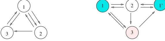
Remark 5.1. (a) Note that when c₁ c₂, any input arrow in I(c₂) with tail cell c₁ leads to a self-coupling arrow in the quotient. If c₁ and c₂ are distinct -equivalent cells having equivalent arrows with the same head cell d, then multiarrows will be present in the quotient network, where amultiarrowis a set of several edge-equivalent arrows between two given cells. For example, see Figure1 (right) and the corresponding quotient network Figure2 (right).

a bijection since I(c) = I(c) and I(d) = I(d). Identity (5.2) guarantees that (2.3) is valid for E-equivalence andβ is an input isomorphism forG. Identity (5.2) also guarantees the converse—every input equivalence onG lifts to one onG.

(c) Since input isomorphisms project, we see that any quotient of a homogeneous network is also a homogeneous cell network. The quotient of the balanced relation of the five-cell example in Figures1and 2(left) shows that this remark is not valid for quotients in the class of networks considered in [10].

We can now generalize Theorem 9.2 of [10] to the multiarrow formalism. The fact that every vector field on the quotient lifts to a vector field on the original network is a major theoretical reason for introducing this new formalism.

Theorem 5.2. Let be a balanced relation on a coupled cell network G. (a) The restriction of a G-admissible vector field to ∆ is G-admissible.

(b) Every G-admissible vector field on the quotient lifts to a G-admissible vector field on the original network.

Proof. (a) The proof of Theorem 5.2(a) is identical to the proof of Theorem 9.2 of [10]. (b) Let cbe a quotient cell and suppose that the dynamics on that cell are prescribed by the ODE

˙

x_c = ˆf_c(x_c, x_T(I(c))),

wherexc ∈Pc =Pc are the internal state space variables andxT(I(c)) ∈PT(I(c)) =PT(I(c)) are

the coupling variables. We can lift this ODE to each cell c that quotients ontocby

˙

xc = ˆfc(xc, xT(I(c))).

(5.3)

Observe that ifc d(orc=d), then there exists an input isomorphismβ :I(c)→I(d). Now

G-admissibility and the fact that input isomorphisms on Gproject onto input isomorphisms on G imply that

ˆ

f_d(x_d, x_T(I(d))) = ˆf_c(x_d, β∗(x_T(I(c)))).

Note that ifc=d, then (5.3) is consistent since fc is invariant underB(c, c). Therefore,

ˆ

f_d(x_d, x_T(I(d))) = ˆf_c(x_d, β∗(x_T(I(d)))),

and the lift (5.3) isG-admissible.

6. Examples of networks. Several examples of networks with interesting properties were presented in [7]. The simplest network with self-coupling is the feed-forward network shown in Figure6. This network has a surprising bifurcation structure. It is shown in [7] that synchrony-breaking bifurcations occur with multiple eigenvalues (and nontrivial Jordan normal form) in codimension one. Suppose that λ is the bifurcation parameter and that Hopf bifurcation occurs at λ= 0. Then this bifurcation leads to periodic solutions whose amplitude growth is the expected λ1/2 in cell 2, but is a surprisingλ1/6 in cell 3.

1

2

3

Figure 6. The three-cell feed-forward network.

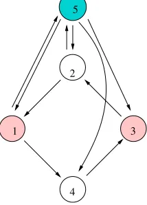
quotient networks can have multiple arrows even when the original network does not. For example the five-cell network in Figure 1 has network 29 in Figure 8 as a quotient network. Another example (that was discussed in [10]) is the balanced coloring in the five-cell network in Figure7whose quotient is the three-cell bidirectional ring (34 in Figure8) withD₃symmetry. In section 8 we prove that every (identical-edge) homogeneous network is a quotient of a homogeneous network without self-coupling and multiple arrows.

1

2

3

4 5

Figure 7. A second homogeneous five-cell network with balanced coloring.

It is also shown in [9] that steady-state, codimension-one, synchrony-breaking bifurcations of the networks in Figure8can occur with simple real eigenvalues, real double eigenvalues with independent eigenvectors (as in the bidirectional ring), real double eigenvalues with nontrivial Jordan blocks (as in the feed-forward network in Figure6), or with complex-conjugate, purely imaginary eigenvalues (as in the three-cell unidirectional ring).

Planar lattice dynamical systems with nearest neighbor coupling have interesting patterns of synchrony. For example, [7] shows that there exists an infinite family of balanced two colorings, almost all of which are not spatially periodic. Wang and Golubitsky [11] classify all balanced two-color patterns with nearest neighbor coupling (NN) and with both nearest and next nearest neighbor coupling (NNN). The classification proceeds by assuming the form of the two-cell quotient and then classifying all balanced colorings that lead to that quotient. In NNN, all balanced relations are spatially doubly periodic (which is strikingly different from the NN), thus illustrating again the importance of network architecture.

estab-1. 1 _{2 3}

2.

1

2 3

3. 1 _{2 3}

4. 1 _{2 3}

5. 2

1 3

6. 2

1 3

7. 1 3 2 _8. 2

1 3

9. 2

1

3 _10. 2

1

3 _11. 2

1

3 _12. 1 2 3

13. 1 3 2 _14. 3 1 2 _15. 1 2 3 _16. 2

1 3

17. 1 3 2 18. 2 1 3 _19. 2 1 3 _20. 2

1 3

21. 2

1

3 _22. 1 2 3

23. 2

1

3 _24. 1 2 3

25. 3 1 2 _26. 1 3 2

27. 1 3 2

28. 1 2 3

29. 2

1

3 _30. 1 3 2

31.

1

3 2 _32.

1 2 3

33.

1 2

3 _34.

1 2 3

Figure 8. Homogeneous three-cell networks with two input arrows at each node from[9].

suf-ficiently small admissible perturbations. In this section we prove that patterns of synchrony associated to hyperbolic equilibria are rigid precisely when they are balanced. Thus, in cou-pled cell networks, the local assumption of rigidity for patterns associated to one equilibrium for each of a small but open set of vector fields implies the global invariance of a polydiagonal subspace for all admissible vector fields. We conjecture that a similar statement is valid for hyperbolic periodic states, but we are currently unable to prove this conjecture.

Let x₀ = (x0₁, . . . , x0_N) ∈ P. Define the equivalence relation ≡x₀ by c ≡x₀ d if and only

if c ∼C d and x0_c = x0_d. (This notation does not conflict with our previous use of ≡c in the proof of Theorem 4.3, which was temporary notation for that proof.) Suppose that we color two cells c and d the same color if and only if c ≡x0 d. Then this coloring is the pattern of

synchrony associated to x₀. Note that

∆_≡x0 ={x∈P :xc =xd if c≡x0 d}

is the smallest subspace of P that contains all points with the same pattern of synchrony.

Definition 7.1. Let x₀ ∈ P be a hyperbolic equilibrium of a C1-admissible cell system. The equivalence relation ≡x₀ isrigid if in eachC1 perturbed admissible system the hyperbolic equilibrium near x₀ remains in ∆_≡x0. We also say that the pattern of synchrony defined by

x₀ isrigid.

Strong admissibility. In Theorem 7.6 we prove that only those patterns of synchrony that are generated by balanced relations are rigid. We prove this theorem by showing that rigid patterns of synchrony lead to flow-invariant subspaces. The following is a key idea in the proof.

Definition 7.2. A mapG:P →P is stronglyadmissible if G_c(x) =G_c(x_c) for every cell c

and Gc =Gd for every pair of cells where c∼C d.

A strongly admissible mapGis admissible sincec∼I dimpliesc∼C dand henceGc =Gd.

Lemma 7.3. Let F :P →P be admissible and let G:P →P be strongly admissible. Then

F◦Gand G◦F are admissible.

Proof. Both (F◦G)c and (G◦F)c are functions defined onPc×PT(I(c)). That is,

(G◦F)c(xc, xT(I(c))) = Gc(Fc(xc, xT(I(c)))),

(F◦G)_c(x_c, x_T(I(c))) = F_c(G_c(x_c), G_T(i1)(x_T(i1)), . . . , G_T(is)(x_T(is))),

where I(c) ={i₁, . . . , is}.

Letβ :I(c)→I(d) be an input isomorphism in B(c, d). OrderI(d) ={j₁, . . . , js}so that

β(i_k) =j_k. It follows from the definition of input isomorphism thatc∼IdandT(i_k)∼C T(j_k) for each k. Hence,F_c =F_d,G_c=G_d, and G_T(ik)=G_T(jk).

We claim that both (F◦G)_c and (G◦F)_c are β related to (F◦G)_d and (G◦F)_d. To verify this point for G◦F, compute

(G◦F)d(xd, xT(I(d))) = Gd(Fd(xd, xT(I(d))))

= G_d(F_c(x_d, β∗x_T(I(d)))) = Gc(Fc(xd, β∗xT(I(d))))

Thus G◦F is admissible. It also follows that

(F◦G)_d(x_d, x_T(j1), . . . , x_T(js)) = F_d(G_d(x_d), G_T(j1)(x_T(j1)), . . . , G_T(js)(x_T(js)))

= Fc(Gd(xd), GT(j1)(xT(j1)), . . . , GT(js)(xT(js)))

= F_c(G_c(x_d), G_T(i1)(x_T(j1)), . . . , G_T(is)(x_T(js)))

= (F◦G)c(xd, xT(j1), . . . , xT(js)).

Thus F◦Gis also admissible.

Definition 7.4.Let be an equivalence relation. A pointx= (x₁, . . . , xN)∈∆ isgeneric

if x_i=x_j for i∼C j implies that i∼j.

Observe that generic points are open and dense in ∆.

Lemma 7.5.Let be an equivalence relation on cells. Letx₀ be a generic point in ∆ and

let y₀ be any point in ∆. Then there exists a strongly admissible map G:P →P such that

G(x₀) =y₀.

Proof. Let x₀ = (x₁, . . . , x_N) and y₀ = (y₁, . . . , y_N). We need to choose functions G_c

(where Gc =Gd wheneverc∼C d) so that

G_c(x_c) =y_c.

(7.1)

Conditions (7.1) are incompatible only when c ∼C d, xc = xd, and yc = yd. When these

conditions are compatible we can always choose strongly admissible interpolation functions

G_c to satisfy (7.1). The facts thatx₀, y₀ ∈∆ and x₀ is generic ensure that conditions (7.1) are compatible because xc =xdimplies yc =yd.

Perturbation spaces and hyperbolic equilibria. Letx₀∈P. Form the subspace

Wx0 ={p(x0) :pis admissible}

consisting of all points obtained from x₀ by applying an admissible map. Let ∆ ⊂ P be the smallest flow-invariant subspace that contains the point x₀. Flow-invariance implies that ∆ = ∆x₀ for some balanced equivalence relation x0. The balanced equivalence relation

x0 is the coarsest for which x0 ∈∆x0. Since ∆x0 is flow-invariant, x0 ∈ ∆x0, and p is admissible, it follows that p(x₀) ∈ ∆_x

0. Thus, Wx0 ⊂ ∆x0. Equality need not hold, in general. However, equality does hold when the pattern of synchrony defined by a hyperbolic equilibrium x₀ is rigid.

Theorem 7.6. The equivalence relation ≡x₀ determined by the hyperbolic equilibrium x₀ is rigid if and only if ≡x₀ is balanced. Moreover, in this case, ≡x₀=_x0 and

Wx0 = ∆≡x₀ = ∆x₀.

(7.2)

Proof. Let x₀ ∈ P be a hyperbolic equilibrium for a C1-admissible vector field f and assume that ≡x₀ is a balanced equivalence relation. It is straightforward to show that ≡x₀ is rigid. Hyperbolicity implies that every small admissible C1 perturbation g of f will have a unique hyperbolic equilibrium y₀ nearx₀. Since ∆x₀ is flow-invariant, uniqueness implies

To prove the converse, we assume that≡x₀ is a rigid equivalence relation. By the definition of ≡x₀,x₀ is generic in ∆_≡x

0. It follows from Lemma 7.5that

∆_≡x

0 ⊂Wx0. (7.3)

We claim that ∆_≡x

0 =Wx0. To verify this claim, letpbe an admissible vector field. Consider the perturbation fε =f+εp and denote by xε the perturbed hyperbolic equilibrium for fε.

So

fε(xε) = 0.

(7.4)

Since rigidity implies xε∈∆≡x0, it follows that

d

dεxε

ε=0 ∈

∆_≡x 0.

Differentiating (7.4) with respect toεand evaluating atε= 0 yield

0 = d

dε(f(xε) +εp(xε))

ε=0

= (Df)_x0 d

dεxε

ε=0

+p(x₀).

Thus p(x₀)∈(Df)x0(∆≡x0); that is, Wx0 ⊂(Df)x0(∆≡x0). In view of (7.3), we obtain

∆_≡x0 ⊂Wx0 ⊂(Df)x0(∆≡x0). (7.5)

Since the vector space ∆_≡x0 is finite-dimensional, (7.5) implies that the inclusions above are all equalities, particularly W_x0 = ∆_≡x0.

Next we show that ∆_≡x

0 is flow-invariant for all admissible vector fields. It then follows from Theorem 4.3 that ≡x₀ is a balanced relation, as desired. Let y ∈ ∆_≡x0 and q be an admissible vector field. We must show that q(y)∈∆_≡x0. By Lemma7.5,y=G(x₀) for some strongly admissible vector field G, and thereforeq(y) =q◦G(x₀). By Lemma 7.3,q◦Gis an admissible field, and therefore q(y)∈Wx0 = ∆≡x₀.

Finally, we verify the moreover part of the theorem. Since ∆_≡x0 is flow-invariant, it follows that ∆_x

0 ⊂∆≡x0. Since Wx0 ⊂∆x0, (7.2) follows. Hence≡x0=x0.

8. Identical-edge homogeneous networks. An identical-edge homogeneous cell network

G is a homogeneous network in which all edges inE are equivalent.

Proposition 8.1. Every quotient of an edge homogeneous network is an identical-edge homogeneous network.

Proof. This statement follows directly from section5 (D) and Remark5.1.

Proposition 8.2. Every edge homogeneous network is the quotient of an identical-edge homogeneous network without multiple identical-edges or self-coupling.

Proof. We begin by showing that if some cell in anN-cell network, say, cell 1, hasm self-couplings, then we can enlarge the network to an (N +m)-cell network, having the original network as a quotient, so that the enlarged network has no self-couplings in cells residing in the pullback of cell 1. Add arrows and cells to the enlarged network as follows.

(2) For each arrow in the original network with head cell 1 and tail cell i, where i= 1, add medge-equivalent arrows with tail celli, where one of the new arrows terminates in each of the m new cells.

(3) Each pair of the m+ 1 cells in the preimage of cell 1 has identical arrows with head in the first cell of the pair and tail in the second cell of the pair.

Note that all arrows starting from one of the m new cells terminate in cell 1. In particular, none of them+ 1 cells in the preimage of cell 1 have self-coupling arrows. In the new network, assign all cells in the preimage of cell 1 the same color and all other cells different colors. This coloring is balanced and yields the original network as a quotient network. See Figure9. Therefore, we can enlarge the original network so that it has no self-coupling arrows.

1 2

3

1 2

3 1’

Figure 9. (Left) Three-cell network with self-coupling. (Right) Four-cell enlargement of original system.

Next, we assume that the network has no self-coupling and that there are m identical arrows from cell 1 to cell 2. There is an extended coupled cell network with N +m−1 cells formed by replacing cell 1 with m identical cells and changing arrows as follows:

(1) Each of the m cells replacing cell 1 connects to cell 2 with one arrow. Note that cell 2 receives the same number of arrows from the m copies of cell 1 that it received previously from the single cell 1 in the original network.

(2) Add arrows so that every cell that was connected to cell 1 in the original network is now connected to each of them cell 1’s in the new network.

Note that there are no arrows starting from one of them−1 new cells that terminate in a cell in the original network not equal to cell 2. In the new network, color all cells in the preimage of cell 1 the same color and all other cells different colors. This coloring is balanced and yields the original network as a quotient network. See Figure 10. Proceeding inductively, we can eliminate multiple arrows between cells.

1

2 3

2

3

1 1’

Figure 10. (Left) Three-cell network with multiple arrows. (Right) Four-cell enlargement of original system.

identical-edge homogeneous network, with the feature that well-defined approximate phase shifts and approximate amplitude relations hold near bifurcation.

Suppose that an identical-edge homogeneous network has a balanced relation with two colors. The corresponding quotient network has the form given in Figure 11. Indeed, Propo-sition 8.1 implies that the two cells are input isomorphic and all edges are identical. Such two-cell networks are determined by the number of self-coupling arrows lj on cell j and the

number of edgesm₁≥0 coupling cell 2 to cell 1. Letm₂≥0 be the number of edges coupling cell 1 to cell 2; then homogeneity implies l₁+m₁ =l₂+m₂.

m₂ m₁

1 2

l₁ l₂

Figure 11. The two-cell quotient network.

Wang and Golubitsky [11] use this quotient network (with multiple arrows and self-coupling) to prove that equilibria corresponding to balanced two-colorings may be obtained from a codimension-one steady-state bifurcation from a homogeneous equilibrium; we use the quotient to study Hopf bifurcations.

Proposition 9.1. Suppose that an identical-edge homogeneous network has a balanced rela-tion with two colors and that the quotient network is not feed-forward, that is, m₁, m₂ >0. Then there is a unique type of synchrony-breaking Hopf bifurcation from a synchronous equi-librium that leads to periodic solutions that are synchronous on all cells of the same color and that are approximately one half a period out of phase with all cells of the opposite color. The amplitudes of these periodic signals need not be equal.

Proof. The coupled cell systems have the form

˙

x₁ = f(x₁, x₁, . . . , x₁

l1times

, x₂, . . . , x₂

m1times ),

˙

x₂ = f(x₂, x ₂, . . . , x₂

l2times

, x ₁, . . . , x₁

m2times ),

(9.1)

where x₁, x₂ ∈ Rk. Since {x : x₁ = x₂} is flow-invariant, we can arrange for the robust existence of an equilibrium in this subspace. Moreover, by a change of coordinates, we can assume that the equilibrium is at the origin. LetJ be the Jacobian matrix of this equilibrium. By (9.1)

J = A+l1B m1B

m₂B A+l₂B

,

where A is the linearization of the internal dynamics and B is the coupling matrix. Assume that x₁, x₂ ∈Rk. Letv∈Rk and observe that

J v

v

= (A+pB)v (A+pB)v

and J m1v

−m₂v

= (A+ (l2−m1)B)m1v

−(A+ (l₂−m₁)B)m₂v

1

2

0 10 20 30 40 50 60 70 80 90 100 −0.5

−0.4 −0.3 −0.2 −0.1 0 0.1 0.2 0.3 0.4 0.5

t

Figure 12. (Left) Two-cell homogeneous network. (Right) Half-period out of phase periodic state with different amplitudes obtained by Hopf bifurcation.

wherep=m₁+l₁ =m₂+l₂. Thus, the eigenvalues ofJ are given by eigenvalues of thek×k

matrices A+pB and A+ (l₂−m₁)B. Either matrix can have purely imaginary eigenvalues when k ≥ 2. Critical eigenvalues in the matrix A+pB lead to periodic solutions that are synchronous on all cells, since the synchrony subspace x₁ =x₂ is flow-invariant.

Synchrony-breaking Hopf bifurcations occur if the matrix A+ (l₂ −m₁)B has (simple) purely imaginary eigenvalues±ωi. Letv₀ ∈Ckbe an eigenvector associated to the eigenvalue

ωi. Then Hopf bifurcation can lead to a branch of periodic solutions that to first order in the bifurcation parameter has the form

x₁(t) =m₁Re(eiωtv₀), x₂(t) =−m₂Re(eiωtv₀).

The amplitudes of the time series x₁(t) and x₂(t) are different (unlessm₁ =m₂). Indeed, to first order they are in the ratio m₁ : m₂ near the bifurcation point. The minus sign in x₂

shows that the time series are (to first order) a half-period out of phase.

Example9.2. Consider the two-cell system in Figure 12 (left). This network can be ob-tained as a two-color quotient network of the five-cell network in Figure1(right) by identifying the four pink and white cells as one color and the cyan cell as the other color. The time series of a periodic state obtained by Hopf bifurcation in this network is shown in Figure12(right). Note that the time series from cells 1 and 2 are approximately one half a period out of phase even though the amplitudes of these signals are quite different. The amplitude ratio here is convincingly close to m₁/m₂= 2. This coupled cell system has the form

˙

x₁ = f(x₁, x₂, x₂, λ),

˙

x₂ = f(x₂, x₂, x₁, λ).

The time series in Figure 12 (right) was obtained using f :R2×R2×R2→R2, where

f(y₁, y₂, y₃, λ) = 0 −1

1 0

+ (λ−1)I₂

y₁−(y₂+y₃)− |y1|2y₁−(y₂, y₃)y₁.

A supercritical Hopf bifurcation from the trivial equilibrium at the origin occurs atλ= 0. In the given time seriesλ= 0.1.

Corollary 9.3. Suppose that an identical-edge homogeneous network has a balanced equiva-lence relation with two colors, black and white. If the number of white cells coupled to a white cell is equal to the number of black cells coupled to a black cell, then the synchrony-breaking Hopf bifurcation in Proposition 9.1 leads to robust periodic solutions that are synchronous on cells of the same color and exactly one half a period out of phase with cells of the opposite color.

Proof. Whenm₁ =m₂ (and hencel₁ =l₂) in Proposition9.1, the transposition (x₁, x₂)→ (x₂, x₁) is a symmetry of (9.1) and the bifurcating states have an exact spatio-temporal sym-metry x₂(t) =x(t+T₂), where T is the (minimal) period.

10. Concluding remarks. Primary goals of our research are the study of the types of typi-cal states that can occur in networks of coupled systems of differential equations (synchronous states are one of these) and the study of typical (codimension-one) synchrony-breaking bi-furcations. Any study of genericity must begin with a precise description of the classes of differential equations that are to be considered, and any abstract study of synchrony-breaking bifurcations must begin with a definition of what synchrony means. In this paper and [10] we have set up a framework (based on groupoids) that specifies both the classes of differential equations (associated to a fixed network) and the notion of (robust) synchrony that can occur in that network (balanced relations).

An important observation is that the restrictions of coupled cell systems to polysyn-chronous subspaces are themselves coupled cell systems associated to the quotient network. This restriction has profound and interesting consequences for the generic behavior of polysyn-chronous dynamics. In this paper we have refined the notion of quotient dynamical systems, through the network theoretic conventions of the multiarrow formalism, to the point that genericity arguments on quotient networks now lift to genericity arguments about polysyn-chronous dynamics in the original network.

It is a nontrivial task to compute all balanced relations in a complicated network; never-theless this is a simpler task than that of computing all flow-invariant subspaces for admissible vector fields. In certain instances, such as with certain types of colorings [7, 11], this clas-sification can be completed, and these clasclas-sifications provide interesting information about patterns of synchrony. The work in [7, 9] shows that codimension-one synchrony-breaking bifurcations can be highly nonstandard (and complicated to analyze). A complete theory for synchrony-breaking will require a better understanding of the Jacobian matrices at syn-chronous equilibria (parallel to the representation theory of matrices commuting with a given group action). At present such a theory does not exist, but some initial steps can be found in [3].

Acknowledgments. We wish to thank Ana Dias and the referees for helpful discussions and suggestions.

REFERENCES

[1] H. Brandt_{,Uber eine Verallgemeinerung des Gruppenbegriffes}¨ _{, Math. Ann., 96 (1927), pp. 360–366.}

[3] A. P. S. Dias and I. Stewart,Symmetry groupoids and admissible vector fields for coupled cell networks,

J. London Math. Soc. (2), 69 (2004), pp. 707–736.

[4] A. P. S. Dias and I. Stewart_{,Linear Equivalence and ODE-Equivalence for Coupled Cell Networks,}

submitted.

[5] I. R. Epstein and M. Golubitsky_{,Symmetric patterns in linear arrays of coupled cells, Chaos, 3 (1993),}

pp. 1–5.

[6] D. Gillis and M. Golubitsky_{, Patterns in square arrays of coupled cells, J. Math. Anal. Appl., 208}

(1997), pp. 487–509.

[7] M. Golubitsky, M. Nicol, and I. Stewart_{, Some curious phenomena in coupled cell networks, J.}

Nonlinear Sci., 14 (2004), pp. 119–236.

[8] P. J. Higgins_{,Notes on Categories and Groupoids, Van Nostrand Reinhold Mathematical Studies 32,}

Van Nostrand Reinhold, London, 1971.

[9] M. Leite and M. Golubitsky,Synchrony-breaking bifurcations in homogeneous three-cell networks, in

preparation.

[10] I. Stewart, M. Golubitsky, and M. Pivato,Symmetry groupoids and patterns of synchrony in coupled cell networks, SIAM J. Appl. Dynam. Sys., 2 (2003), pp. 609–646.

[11] Y. Wang and M. Golubitsky,Two-color patterns of synchrony in lattice dynamical systems,

Nonlin-earity, 18 (2005), pp. 631–657.