publisher policies. Please scroll down to view the document
itself. Please refer to the repository record for this item and our
policy information available from the repository home page for
further information.
To see the final version of this paper please visit the publisher’s website.
Access to the published version may require a subscription.
Author(s): J. SAI-LAP LAM and DAVID G. DRITSCHEL
Article Title: On the beta-drift of an initially circular vortex patch
Year of publication: 2001
Link to published version:
c
2001 Cambridge University Press
On the beta-drift of an initially circular
vortex patch
By J. S A I-L A P L A M1†AND D A V I D G. D R I T S C H E L2‡
1Department of Applied Mathematics and Theoretical Physics, University of Cambridge, Silver Street, Cambridge CB3 9EW, UK
2Department of Mathematics, University of Warwick, Coventry CV4 7AL, UK
(Received 25 November 1997 and in revised form 27 July 2000)
The nonlinear inviscid evolution of a vortex patch in a single-layer quasi-geostrophic fluid and within a background planetary vorticity gradient is examined numerically at unprecedented spatial resolution. The evolution is governed by two dimensionless parameters: the initial size (radius) of the vortex compared to the Rossby deformation radius, and the initial strength of the vortex compared to the variation of the planetary vorticity across the vortex. It is found that the zonal speed of a vortex increases with its strength. However, the meridional speed reaches a maximum at intermediate vortex strengths. Both large and weak vortices are readily deformed, often into elliptical and tripolar shapes. This deformation is shown to be related to an instability of the instantaneous vorticity distribution in theabsenceof the planetary vorticity gradientβ. The extremely high numerical resolution employed reveals a striking feature of the flow evolution, namely the generation of very sharp vorticity gradients surrounding the vortex and extending downstream of it in time. These gradients form as the vortex forces background planetary vorticity contours out of its way as it propagates. The contours close to the vortex swirl rapidly around the vortex and homogenize, but at some critical distance the swirl is not strong enough and, instead, a sharp vorticity gra-dient forms. The region inside this sharp gragra-dient is called the ‘trapped zone’, though it shrinks slowly in time and leaks. This leaking occurs in a narrow wake called the ‘trailing front’, another zone of sharp vorticity gradients, extending behind the vortex.
1. Introduction
Isolated coherent vortices are ubiquitous in planetary atmospheres, in the oceans and, generally, in rotating, stratified fluids. One of the most striking examples is Jupiter’s Great Red Spot. These vortices appear in various forms, but are most fre-quently monopolar or dipolar. They are characterized by their longevity (lifetimes greatly exceeding their characteristic rotation time) and their ability to withstand the background turbulent fluctuations ever present in real flows. An important con-sequence is that vortices tend to trap and advect fluid particles over lengths much greater than their characteristic size. For vortex dipoles, such non-diffusive tracer transport is enabled by the mutual propagation of the constituent vortex pair while, for monopolar vortices, it may be enabled by an ambient potential vorticity gradient.
† Present address: Department of Mathematics, Hong Kong University of Science and Technol-ogy, Clear Water Bay, Hong Kong.
an idealized background planetary vorticity gradient, namely aβ-plane.
Numerous studies of this topic have been made in the past few decades. Approaches include theoretical (Adem 1956; Flierl 1977; Sutyrin 1987, 1988; Reznik 1990, 1992; Sutyrin & Flierl 1994; Sutyrin & Morel 1997), numerical (McWilliams & Flierl 1979; Meid & Lindemann 1979; Sutyrinet al. 1994) and experimental (Firing & Beardsley 1976; Carnevale, Kloosterziel & van Heijst 1991). Extensive discussions of vortex drift on aβ-plane and the associated Rossby wave radiation can also be found in the past literature (see e.g. Sutyrin 1987, 1988 and McDonald 1998). Nonetheless, a full understanding of the nonlinear flow development up to late times is lacking in our view, and it appears to be beyond analytical treatment.
The purpose of the present work is to provide an accurate picture of this late and complex stage of evolution, and to point out its most salient characteristics. We shall study the circular vortex patch model which, arguably the simplest conceptually, has not yet been adequately examined owing to technical difficulties arising from the vorticity discontinuity at the vortex edge. Sutyrin & Flierl (1994) have examined the short-time behaviour of this model analytically; here we shall present high-resolution numerical results for the long-term behaviour.
The dynamics of an isolated vortex on aβ-plane is governed by two inter-related processes: (i) the generation of a residual (or regular) flow by the redistribution of am-bient potential vorticity within the planetary vorticity gradient, and (ii) the deforma-tion of the vortex (cf. Sutyrin & Flierl 1994). Using a vortex patch model, one can track the detailed movement and deformation of the vortex boundary without encountering the difficulty and ambiguity intrinsic to Gaussian or other (continuously) distributed vortices. The vortex patch model allows one to deduce straightforwardly the flow aris-ing from the vortex and thus to dissociate these two processes for separate analysis.
Owing to the nonlinearity of the governing equations, the long-term evolution of a vortex patch can only be treated by direct numerical simulation. However, in general it is difficult to simulate flows with vorticity discontinuities, since most numerical methods depend on down-gradient diffusion of some sort for stability. Contour dynamics (CD, see Dritschel 1989), which seems to be the only appropriate scheme for this type of problem, is not satisfactory either. The reason lies in its lack of efficiency when a multitude of contours are followed – this is the case for β-plane geometry as we shall see shortly. As a consequence, there has been little previous work on the long-term behaviour of vortex patches on a β-plane. Perhaps the most closely related work is that of Sutyrin & Morel (1997), who studied this problem both analytically and numerically. For their numerical simulations, they used a hyperviscous pseudo-spectral method, which compromised the long-time accuracy of their solutions. In particular, the sharp gradients at the vortex boundary, and those created during the vortex evolution, were not well resolved.
vortex patches with different sizes and strengths on the β-plane. The formulation of the model problem, to be investigated in the context of the equivalent barotropic quasi-geostrophic (QG) approximation, is introduced in §2. A decomposition of the whole flow field into regular and singular parts is described in the second half of this section. These two parts are respectively related to the induced residual flow generated by the redistribution of ambient potential vorticity and by the deformation of the vortex. Details of the numerical implementation of the CASL algorithm for β-plane geometry are discussed in§3. There, the evolution of the potential vorticity field is illustrated in several representative cases. Many well-known features, such as tripolar structures and the trailing front, are here obtained at extraordinarily high resolution. In §4, we present quantitative results for the vortex trajectories, while in §5 we examine the vortex deformation and its relation to the stability of the local vorticity distribution. In§6, we focus on the development of sharp potential vorticity gradients at the periphery of the trapped zone and in the ‘trailing front’ or wake of the vortex. Our conclusions are presented in §7.
2. Mathematical formulation
2.1. Model problem
We examine the evolution of an initially circular vortex patch moving on a β-plane. Letβbe the planetary vorticity gradient,Rdthe Rossby deformation radius andψ the
streamfunction. The equivalent barotropic QG equation (Pedlosky 1987), describing the material conservation of QG potential vorticity (denoted as PV hereinafter) in a single-layer shallow-water fluid is given by
Dq Dt ≡
∂q
∂t +J(ψ , q) = 0, (2.1)
where
q=ω+βy, ω= (∇2−R−2
d )ψ. (2.2)
J(. , .) and ∇2 are the Jacobian and horizontal Laplacian operators respectively. The
horizontal flow u≡(u, v) is non-divergent and thus can be expressed as
u=−∂ψ ∂y, v =
∂ψ
∂x. (2.3)
Cartesian coordinates are adopted with positivexeastward and positiveynorthward. Note that the PV drives the entire flow evolution; its instantaneous distribution wholly determines the velocity field, and this field advects the PV to the next instant of time. Although this ideal property does not carry over in its entirety to the unapproximated equations governing atmospheric and oceanic motions, it is often an excellent approximation (see Hoskins, McIntyre & Robertson 1985). The real limitation of the present model is the use of just one layer.
The initial condition considered consists of a circular vortex patch with uniform PV anomaly:
ω(x, y)t=0 =
(
ω0= constant if
p
x2+y2 < R;
0 otherwise, (2.4)
(2.5) constitute the complete mathematical description of our model problem. The evolution for other values of βand Rd can be related to this model form by a simple
rescaling on the characteristic Rossby wave time and length scales:
T = (βRd)−1, L=Rd, (2.6)
which leads to the following relationships:
ω0= ω
∗
0
βRd, R =
R∗
Rd, (2.7)
between the original parameters (marked with an asterisk) and the model parameters. Note that there are two different intrinsic time scales in this problem. One is the fast time scale associated with the swirling velocity field due to the PV anomaly 4π/ω0.
The other is the slow time scale associated with the Rossby wave propagationT. The latter time scale characterizes the propagation of the vortex, and here we consider tT.
2.2. Flow decomposition We decompose the flow as follows:
q=qs+qr, ψ=ψs+ψr (2.8)
where
qs= (∇2−1)ψs, qr = (∇2−1)ψr+y. (2.9)
The quantity qs is the PV anomaly of the vortex patch, i.e.
qs(x, y, t) =ω0χD(x, y) (2.10)
where D specifies the region which the vortex patch occupies at time t and the characteristic function χD equals 1 insideD and 0 elsewhere. Conventionally,qs and
qr are termed the singular and regular parts (ψs and ψr likewise) although here qs is
not strictly singular in the sense that its value is bounded throughout the domain. The motion of the vortex boundary ∂D is described by dx/dt = u(x, t) for all
x≡(x, y)∈∂D. Hence, from (2.1) and (2.4), we have
qr(x, y)|t=0=y (2.11)
and
Dqr
Dt = 0. (2.12)
Equation (2.12) shows that the quantityqr is a pointwise conservative field generating
the regular flow ψr in the presence of the planetary PV gradient. This decomposed
3. Numerics
3.1. The algorithm
The piecewise-constant nature of the initial condition (2.4) poses difficulties for conventional methods such as finite difference methods (cf. McWilliams & Flierl 1979) and spectral methods (cf. Sutyrin et al. 1994). In fact, the real difficulty lies not so much with the initial conditions but rather with the inviscid character of the flow. In time, even smooth initial conditions tend to develop practically infinite PV gradients. Conventional methods simply cannot deal with such situations efficiently; significant dissipation must be used to control numerical stability, which implies a continuous erosion of sharp gradients as they try to form (see Mariotti, Legras & Dritschel 1994 and Yao, Dritschel & Zabusky 1995). This erosion can have a significant influence on solution accuracy, as demonstrated recently by Dritschel, Polvani & Mohebalhojeh (1999).
The difficulty of maintaining numerical accuracy when sharp gradients form can be avoided by using contour dynamics (CD, Dritschel 1989), in which dissipation is produced by surgery only and is negligibly small. However, for complex flows, such as considered here, where many auxilliary contours are needed to represent the background planetary vorticity, CD is simply not efficient. Its cost grows with the square of the number of points n used to represent the contours. To improve the efficiency of CD, Dritschel & Ambaum (1997) combined parts of CD with a standard pseudo-spectral method. In this hybrid algorithm, called the ‘contour-advective semi-Lagrangian’ (CASL) algorithm, the slowest aspect of CD – computing the velocity on the contour points – is replaced by a two-step procedure: first, the velocity field is obtained on a regular grid by a conventional spectral approach, and second, this velocity is interpolated onto the contour points. The spectral approach is generally much faster at computing the velocity field, which here amounts only to inverting the Helmholtz operator on the field of PV and takingxandyderivatives of the resulting streamfunction. This requires the PV at grid points, and this PV is obtained using a fast-fill algorithm at O(n) cost. The evolution of the PV field is computed by contour advection, i.e. by solving a system of o.d.e.’s for the contour points, thereby avoiding the CFL stability constraint associated with grid-based advection. The upshot is that the total numerical cost isO(n) plusO(N2), whereN is the grid resolution, compared
withO(n2) in CD. In practice, modest grid resolution can be used while still achieving
high overall accuracy.
As mentioned in the previous section, we shall deal directly with the decomposed system (2.10)–(2.12), rather than with the original system (2.1)–(2.5). This amounts to advecting the vortex boundary ∂D and the isolines of qr by the total velocity field u= (u, v), where
u=− ∂
∂y(ψs+ψr), v= ∂
∂x(ψs+ψr) (3.1)
and where the streamfunctions ψs and ψr are found from (2.9).
The flow is simulated within a doubly periodic square domain of size [−l, l], with l = 5πhere. The coarsest horizontal grid resolution is ¯nh= 512 in each direction, and
the PV contour-to-grid conversion is done on a grid twice as fine in each direction (mg = 2). Surgery, or the removal of fine-scale filamentary PV, is applied at the
cut-off scale δ = 1×10⁻³ to control the growth of number of contour nodes in
x
t = 0
dβ
Figure 1.An isometric view showing the initial distribution of PV before (dotted) and after (solid) discretization, as given by equation (3.4). The shaded surfaces correspond to the PV discontinuities introduced by discretization, i.e. theβ-contours.
To be compatible with the CASL algorithm, the initial (linear) distribution of qr
(2.11) must be discretized into a finite number of steps – see figure 1. The simplest way to do this is to use a certain number, saynβ, of equally spaced steps. These are
zonal contours placed at the following positions: y= (k− 1
2)dβ−l, k= 1, . . . , nβ, (3.2)
where
dβ = n2l
β. (3.3)
This corresponds to a discretized qr distribution of the form
qr(x, y)|t=0 =
y dβ +
1 2
dβ (3.4)
where [.] denotes the integer part. Figure 1 illustrates the initial distribution of total PV,q, before and after discretization. Whileqr is noty-periodic,qr−y is, and this is
all that is required to obtain ψr.
The number of β-contours, nβ, as well as the values of ¯nh, mg and δ, limit the
accuracy of the numerical simulation. Finite nβ introduces a source of error which
can be kept small if
l
nβR 61 and
l
nβ|ω0| 1, (3.5a,b)
or, in terms of the dimensional quantities l∗, R∗,ω∗
0 and β (see (2.7)), if
l∗
nβR∗ 61 and
βl∗
nβ|ω∗0| 1. (3.6a,b)
Vortex R ω0 nβ l/nβR l/nβ|ω0| Figure Behaviour
A 0.25 20 150 0.42 5.2×10⁻³ 2 weak
B 80 1.3×10⁻³ 3 moderate
C 240 4.4×10⁻⁴ 4 strong
D 1.0 5 50 0.31 6.3×10⁻² 5 weak
E 20 1.6×10⁻² 6 moderate
F 80 4.9×10⁻³ 7 strong
Table 1.Parameters used in the numerical simulations. The parameters common to all simulations are:l= 5π, ¯nh= 512,mg = 2 andδ= 1×10⁻³. The classification of the characteristic behaviour is
based on observation.
Of course, in principle one would like to choose a very large value of nβ, but in
practice the limited computational resources available force a compromise between accuracy and efficiency. In the present work, we have compared simulation results for increasing nβ until the contour shapes converge to within a desired accuracy.
Empirically, it suffices to have l/nβR ∼1 and l/nβ|ω0| ∼10−1 for an error tolerance
consistent with the prescribed values of ¯nh, mg and δ (see Legras & Dritschel 1993
for further remarks; see also Dritschel & Ambaum 1997).
Finally, the finite domain size constrains the duration over which the simulations can reliably approximate the vortex motion in an unbounded domain. This duration is chosen to be the time that it takes the fastest Rossby wave to propagate across the
computational domain, or t = 28 here. Since the maximum wavelength admissible
to the square domain is 2l, i.e. the length of its edge, the actual non-dimensional maximum Rossby group velocities are cg,max= 1/(1 + (π/l)2)≈0.9615 westward and
cg,max/8 eastward in the present study wherel= 5π.
3.2. Numerical results
Direct numerical calculations have been performed to investigate the long-term be-haviour of vortex patches over a range of sizesR and strengths ω0. Only two sets of
representative numerical simulations are described here: R= 0.25 and 1.0, each with three different strengths ω0. A list of the parameters for each simulation is given in
table 1, and the corresponding PV evolution is given in figures 2 to 7. Note that, in these figures, only a fraction of the β-contours used is shown.
Just as with distributed cyclonic vortices, the vortex patches considered here demon-strate a characteristic northwest migration on theβ-plane, i.e.β-drift. This migration is accompanied by Rossby wave radiation, particularly in the wake of the vortex. Both of these phenomena are caused by the redistribution of ambient PV. Under the influence of the swirling singular (or vortical) flow ψs, β-contours initially begin to
wrap around the vortex. The corresponding redistribution of ambient PV leads to the development of a dipolar asymmetry in the regular flow ψr, a pattern termed
‘the β-gyres’ (Peng & Williams 1990; Smith & Ulrich 1990). These β-gyres in turn propel the vortex zonally and meridionally. In time, higher modes of asymmetry emerge in ψr. These asymmetries generate Rossby waves in the wake and perturb
Figure 2.A CASL simulation of the evolution of vortex A (R= 0.25 andω0= 20) on aβ-plane. The frames show the momentst= 7.0,14.0,21.0 and 28.0, from top to bottom. The domain shown is [−l, l]×[−0.25l,0.75l], in which only one out of every threeβ-contours are shown for brevity.
4. Beta-drift
Figure 3.Same as figure 2, except thatω0= 80, i.e. vortex B.
Figure 4.Same as figure 2, except thatω0= 240, i.e. vortex C.
centroid (x0(t), y0(t)) as the vortex centre. This choice is natural because it results in
vanishing first-order moments in an expansion of the velocity field exterior to the vortex (Dritschel 1993).
Figure 5.Same as figure 2, except thatR= 1.0 andω0= 5, i.e. vortex D. For this bigger vortex patch, allβ-contours are shown.
Note that the boundary deformation, at least before surgery, does not have a direct impact on the motion of the vortex centre. This is because the singular (or self-induced) flow ψs vanishes at the centroid. The trajectory is thus determined by
the accumulated effect of the regular flow ψr only.
Figure 6.Same as figure 5, except thatω0= 20, i.e. vortex E.
On the other hand, the meridional speed is not monotonic; vortices of intermediate strength exhibit the largest meridonal speed (see vortices B and E). This remarkable phenomenon was also noted by Rasmussenet al. (1994, figure 2b) and Sutyrin et al. (1994) for Gaussian vortices. The latter authors attributed this phenomenon to the interaction between the vortex and radiating Rossby waves.
Figure 7.Same as figure 5, except thatω0= 80, i.e. vortex F.
1.0
0.5
0
ω0 = 240 (C) y
0
π
–10 –8 – 6 – 4 –2 0
x0/π
1.0
0.5
0
ω0 = 80 (F)
–10 –8 – 6 – 4 –2 0
x0/π
Figure 8.The trajectories of the vortex centre for (a)R= 0.25 (vortices A to C) and (b)R= 1.0 (vortices D to F). The crosses (+) specify the instantaneous positions of the vortex centre at time intervals of 7 nondimensional units. The triangles (4) and the diamonds () on the axes indicate the corresponding zonal and meridional displacement of a point moving at both maximum zonal (cg,max) and maximum meridional (0.25) Rossby group speeds. Note that the fourth diamond is
outside the axis frame.
5. Deformation and instability
Perturbations to the initially circular vortex boundary develop as soon as the regular flow ψr is established. Here, the leading-order, elliptical boundary deformation of a
vortex is quantified in terms of the aspect ratio λ(61) of an analogous ellipse with identical second-order spatial moments (Legras & Dritschel 1991). The variation of λ with time t for our simulations is displayed in figure 9. By comparing parts (a) and (b), one may observe that small vortices (R = 0.25) in general remain circular for longer than do large vortices (R = 1.0). For each value of R, it is also found that the stronger vortices are less vulnerable to deformation. This is logical, as strong compact vortices are less affected by the strain arising from the surrounding Rossby wave field.
Let us now restrict attention to the large vortices first. The weakest such vortex (vortex D) deforms rapidly and is soon torn apart by the straining field present inψr.
The other two stronger vortices (vortices E and F), however, are able to maintain their identity throughout the simulations. An important feature to note for these vortices is the formation of an annulus of fluid which moves along with the vortices. This annulus of fluid is called the trapped zone (cf. Korotaev & Fedotov 1994). It consists of relative vorticity of the opposite sign acquired as the vortex displaces meridionally (a consequence of the conservation of PV). As a result, the vortex becomes shielded, i.e. its net circulation (including the annulus) tends to zero in time.
At this stage of evolution, the vortex evolves in a quasi-steady way. In time, the vortex may deform into an ellipse and may suddenly destabilize, fragmenting into smaller structures. This behaviour, as shown below, can be understood by considering the linear stability of the vortex in the absence of the β-effect, following an earlier analysis by Flierl (1988).
0.8 0.6 0.4 0.2 0 (a)
ω0 = 20 (A)
ω0 = 20 (A)
ω0 = 20 (A)
ω0 = 80 (B)
λ
10 20 30
t
(b)
ω0 = 20 (E)
ω0 = 5 (D)
ω0 = 80 (F) 1.0
ω0 = 240 (C)
0.8
0.6
0.4
0.2
0 10 20 30
t 1.0
Figure 9.The temporal variation of the aspect ratioλof the vortex boundary for (a)R= 0.25 (vortices A to C) and (b)R= 1.0 (vortices D to F).
centre such that
x−x0= (rcosθ, rsinθ), (5.1)
wherex= (x, y) andx0= (x0, y0). The regular partqr(t, r, θ) is expanded as follows:
qr−y=q0(t, r) +
∞
X
n=1
(qc
ncosnθ+qnssinnθ). (5.2)
The structure of the first few modes (q0, qc1 and q1s) for vortices B and C is given
in figure 10. Note the steep jump in q0 at the time shown. This is anticipated to be
a general feature as discussed in the next section. Between the steep jump and the origin,q0 resembles a flat-bottomed well, where the PV has been homogenized by the
rapid swirling flow in ψs. It is reasonable, therefore, to identify the position of this
steep jump as the trapped-zone radius ˜R.
In practice, we define ˜R to be the radius from the vortex centre to the mid-point of two consecutive radial nodes r1 < r2, separated by a distance equal to the size of
the fine underlying grid, where
q0(r2)−q0(r1) (5.3)
is maximum. (If such a mid-point is not unique, we choose the one furthest from the vortex centre. This is sufficient because q0 is generally smooth outside the trapped
zone.) The average relative vorticity acquired inside the trapped zone is approximated by minus y0 (this is an excellent approximation, as can be seen by comparing the
flat-bottom value of q0 in figure 10 with the corresponding position of the vortex
centre in figure 8a).
The Appendix describes the derivation of the linear stability criterion for various modes of boundary perturbation. Basically it repeats the calculation of Flierl (1988), except that Flierl considered a barotropic basic flow (Rd =∞). In our present work,
both the basic flow and the disturbances are equivalent barotropic (Rd is finite).
Figure 11 shows the part of the (y0/ω0,R/R˜ )-plane which is unstable to m = 2
–2 –3 – 4 (a) 0 2.0 r/π (b)
0.5 1.0 1.5 2.5
q0 qc 1 qs 1 – 3 0 2.0 r/π
0.5 1.0 1.5 2.5
q0 qc 1 qs 1 –2 –1
Figure 10.The Fourier decomposition (see (5.2)) of the regular partqr for (a) vortex B and (b)
vortex C at time t= 21.0. The vertical dotted line indicates the trapped-zone radius ˜R which is defined to be the radial distance from the vortex centre with the maximum gradient ofq0.
(a)
y0
ω0
(b)
2 3 4
R/R 0.30
1 0
t = 28
t = 7
t = 14
m = 3
m = 3
m = 3
m = 2
t = 35
t = 21 0.25 0.20 0.15 0.10 0.05 0.05 0.05
m = 3
m = 3
m = 3
2 3 4
R/R 1 0 0.25 0.20 0.15 0.10 0.05 0.05 0.05 ˜ ˜
t = 21
t = 14
t = 7
m = 2
m = 2
m = 2
Figure 11.Stability curves form= 2 (bold) andm= 3 (thin) wavenumbers for (a) vortex A and (b) vortex E. The regions enclosed by these curves are unstable. Circles (◦) joined by dotted lines are obtained from the numerical simulations.
(vortex A) while 11(b) shows the case R = 1.0, ω0 = 20 (vortex E). It should be
noted that the value of ˜R calculated by our method is inaccurate at the beginning of the simulation when the trapped zone has not been well established. This method also breaks down when the vortex suffers severe boundary deformation. This is the reason for the abrupt decrease and subsequent fluctuation in the value of ˜R/Raround y0/ω0 ≈0.13 in figure 11(b). This sharp decrease, in fact, corresponds to the moment
0 1.4 4.0 6.0
7.0 8.6 9.0 9.6
10.2 12.0 13.8 16.4
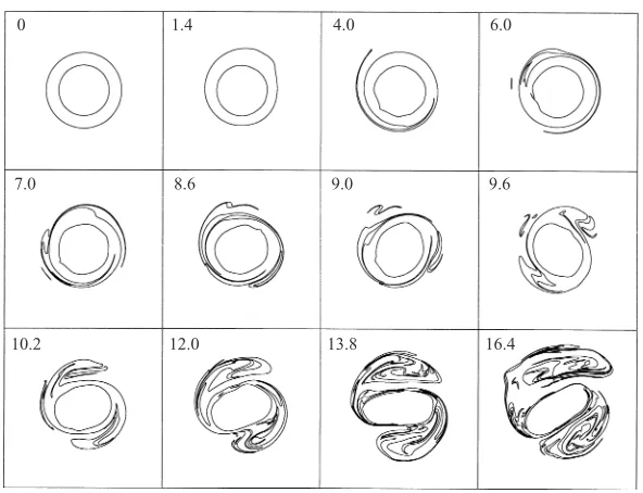
Figure 12. The detailed development of the rotating tripolar structure (first shown in figure 6) is revealed with the help of an initially circular passive tracer contour of radius r = 1.5 (outer contour). The inner contour is the vortex boundary.
Figure 11(b) shows that vortex E has traversed a large part of the unstable region for the elliptical (m= 2) mode. This vortex severely deforms and a rotating tripolar structure emerges, a manifestation of the mode-2 instability (cf. Carton & Legras 1994). This phenomenon was also observed for isolated Gaussian vortices moving on aβ-plane, as noted by Sutyrinet al. (1994). The detailed development of the tripolar structure is displayed in figure 12 with the help of an outer passive tracer contour. The tripolar rotation and the elliptical vortex core together cause the vortex to wobble, as seen in the wavy shape of its trajectory in figure 8. By contrast, the small vortex A (of the same strength) in figure 11(a) falls into the unstable region form= 2 only in its late stage of evolution. Figure 2 shows that this vortex remains stable untilt= 28 (last frame shown), when a small tripolar structure emerges.
It should be remarked that the actual evolution of the vortex is intrinsically nonlinear. A slight discrepancy is therefore expected between the actual onset of instability and that predicted by linear theory. Moreover, that theory neglects β.
6. Formation of steep PV gradients
As shown in figure 10, a steep PV gradient in q0 exists near the periphery of the
trapped zone. This trapped zone is formed by the entrainment of fluid from the vicinity of the drifting vortex. It moves along with the vortex and forces the external iso-PV contours (β-contours) out of its way. Since such contours are material curves, they cannot be crossed by any of the fluid particles advected along with the vortex. Thus, as the vortex approaches, these contours embrace the trapped zone and are subsequently dragged along with it (but not trapped by it). The repeated engulfment of the trapped zone by these external iso-PV contours results in the development of a steep PV gradient.
[image:18.595.148.444.126.353.2]t = 7.0
t = 14.0
t = 21.0
t = 24.0
t = 26.0
t = 28.0
t = 30.0
Figure 13.The formation of the trailing front and the sharp PV gradient around the trapped zone is illustrated by the evolution of two selectedβ-contours, namelyy= 0.42πand 1.5π, for the vortex B (R = 0.25 and ω0 = 80). The closed contour is the vortex boundary. The domain is shifted by 0.5π eastwards. Att= 21 and 24, we see that these twoβ-contours, being pushed northwards by the vortex, approach each other. Parts of these contours become coincident and indistinguishable subsequently, indicating the presence of very large PV gradients there.
The formation of these steep PV gradients is vividly depicted in figure 13, which shows the detailed evolution of selected β-contours for vortex B. It is remarked that the mechanism described above is applicable to distributed vortices as well. Steep PV gradients are anticipated to form in any inviscid evolution of an isolated vortex on theβ-plane.
7. Conclusions
The long-term inviscid evolution of an initially circular vortex patch on aβ-plane has been examined at unprecedented resolution using the CASL algorithm. The successful application of this algorithm demonstrates its effectiveness and robustness for simulating geophysical flows having a non-uniform ambient PV distribution. Two criteria have been developed to ensure accurate flow simulations. The first is that the spacing between ambient PV contours must be small compared to the vortex diameter. The second is that the PV jump across each ambient PV contour must be small compared to the vortex PV anomaly. These criteria, summarized in (3.5) or (3.6), serve as a fundamental guideline for discretizing any initial continuous PV profile.
The flow decomposition described in this work allows us to split the whole flow field into two parts. Theregular part corresponds to the flow induced by the redistribution of ambient PV. The singular part corresponds to the flow generated by the vortex. The singular flow is solely determined by the vortex, or even just its boundary for a vortex patch. This decomposition turns out to be natural for the implementation of the CASL algorithm. It also appears to be useful for the analysis of the vortex motion and deformation.
In our analysis, we have used the centroid as the vortex centre, in terms of which we have obtained the trajectories of the vortices as a function of their size and strength. We have found that the zonal speed of a vortex increases with its strength. However, the maximum (average) meridional speed occurs for vortices of intermediate strength (for the time span considered in our simulations). The latter conclusion was also reached in previous studies of distributed (Gaussian) vortices.
Unlike previous studies, we have considered the effect of vortex size. Large vor-tex patches have been found to deform more readily than small vortices. Moreover, vortices acquire an annular region of trapped fluid (called the trapped zone) which cancels the circulation of the vortex core. This trapped zone shrinks in size but be-comes more intense while the vortex displaces meridionally. Following and extending the results of Flierl (1988), a linear stability analysis for shielded vortices has been performed for β = 0. Despite not including the ambient PV gradient explicitly, this analysis is nevertheless capable of explaining the emergence of tripolar structures in our simulations via the destabilization of an elliptical boundary perturbation.
Apart from the slight dissipation due to fine-scale surgery, the CASL algorithm is essentially inviscid. It has enabled us to capture the development of abrupt PV gradients around the trapped zone and in the trailing front making up the wake of the vortex. These virtual PV discontinuities are formed by the wrapping of external iso-PV contours (β-contours) around the trapped zone as the vortex tries to propagate through them. Without viscosity, these sharp gradients persist and the background planetary vorticity is permanently modified. Since this mechanism is also applicable to distributed vortices, steep PV gradients are expected to be a general feature of vortex motion on the β-plane.
b
qa
qb
Figure 14.Cross-section of the two-level circular vortex patch, approximating the local PV field observed in our numerical simulations.
vorticity gradient undermines the use of such smooth gradients in conjunction with strong vortices. If no mechanism, such as viscosity, is available to restore a smooth gradient, the effect of many vortex passages through a region of varying planetary vorticity must be to focus the gradients into narrow regions, i.e. into jets. This may explain the predominance of such jets in the oceans, the atmosphere and other planetary atmospheres.
Finally, it is remarked that a quasi-steady drift speed has been observed for sufficiently strong vortices, shortly after the simulation commences. Koroteav & Fedotov (1994) gave approximate analytical formulae for the zonal and meridional drift speed of an isolated Gaussian vortex (see their equations (4.30) and (4.31)). They expressed these speeds in terms of the slow-varying meridional displacement of the vortex. In their derivation, the domain is divided into two parts by the separatrix of the streamfunction. This separatrix is assumed to be the boundary of the trapped zone. The corresponding inner and outer solutions are then matched along this separatrix or the trapped-zone boundary. This domain decomposition technique is in fact natural to our present problem. As figure 10 in§5 suggests, the flow inside and outside the trapped zone is quite different. An attempt has been made by Lam (1998) to derive corresponding analytical formulae for an initially circular vortex patch. The domain is divided in the same way. A steady solution corresponding to a dipole with a zonal axis is obtained for the inner solution forr <R˜ (cf. equation (7.1) of Sutyrin & Flierl (1994), in whichrM stands for the radius of the outermost contour, instead
of the trapped-zone radius). The outer solution is ‘solved’ by a heuristic argument. Although the inner solution shows a good agreement with numerical calculations, the outer solution is not accurate enough. Efforts are being made to establish a better outer solution. Such predictions of the vortex drift speed are important and worth further research, particularly in the more general context where the ambient PV gradient is non-uniform (e.g. over topographic features in the ocean). They may not only allow us to have a better quantitative estimate of the impact (due to passive tracer transport) of geophysical vortices on their surrounding environment, but may also enhance our understanding of the role played by Rossby wave radiation in the propagation of vortices.
this interesting problem. D. G. D. was supported by a fellowship from the Natural Environment Research Council. The computations were performed on the Hitachi S3600 made available by courtesy of the High Performance Computing Facilities at the University of Cambridge and the High Performance Computing Centre at Maidenhead, UK. The authors would like to thank the anonymous referees for valuable comments and suggesting helpful references.
Appendix
The linear stability criterion (corresponding to equation (3.5) of Flierl 1988) for a circular vortex consisting of two uniform regions of PV (cf. figure 14) on anf-plane can be shown to be
¯
V(a) a −qaIm
a Rd Km a Rd
− V¯(b) b +qbIm
b Rd Km b Rd 2
<−4qaqbIm2
a Rd K2 m b Rd (A 1)
where a and qa are the radius of and the PV jump across the inner contour of the
vortex. Likewise b and qb are defined for the outer contour. The integer m denotes
the azimuthal wavenumber of the boundary perturbation, taken to be proportional to exp (im(θ−σt)) on each contour, whereσdenotes the angular velocity at which the perturbation propagates along both contours of the vortex. The azimuthal velocity
¯
V(r) generated by the unperturbed vortex is determined by
d2
dr2 +
1 r
d dr −
1 R2 d + 1 r2 ¯
V(r) =−qaδ(a−r)−qbδ(b−r) (A 2)
whereδ is the delta function. This implies that ¯
V(a)
a =
b aqbK1
b Rd I1 a Rd
+qaK1
a Rd I1 a Rd
, (A 3)
¯ V(b)
b =
a bqaK1
b Rd I1 a Rd
+qbK1
b Rd I1 b Rd
. (A 4)
Equations (A 3) and (A 4) are the crucial difference between our present treatment and that of Flierl (1988). The latter studied a barotropic vortex subject to baroclinic perturbations and, therefore, the angular velocity along the contours of the vortex used there is a special case of (A 3) and (A 4) withRd→ ∞.
For our present problem, we have
Rd= 1, a=R, qa=ω0, b= ˜R, qb =−y0, (A 5)
in terms of which the stability criterion (A 1) becomes
¯
V(R)
R −ω0Im(R)Km(R)− ¯ V(˜R)
˜
R −y0Im(˜R)Km(˜R)
2
<4ω0y0Im2(R)Km2(˜R) (A 6)
and the angular velocities at the PV discontinuities are ¯
V(R)
R =
ω0K1(R)−
˜ R
Ry0K1(˜R)
most two solutions for y0/ω0 for each value of ˜R/R. Figure 11 shows the stability
curves for wavenumbers m= 2 andm= 3 for vortices A and E.
REFERENCES
Adem, J.1956 A series solution for the barotropic vorticity equation and its application in the study of atmospheric vortices.TellusVIII, 346–372.
Carnevale, C. F., Kloosterziel, R. C. & Heijst, G. J. F. van 1991 Propagation of barotropic vortices over topography in rotating tank.J. Fluid Mech.223, 119–139.
Carton, X. & Legras, B.1994 The life-cycle of tripoles in two-dimensional incompressible flows. J. Fluid Mech.267, 53–82.
Dritschel, D. G.1989 Contour dynamics and contour surgery: numerical algorithms for extended, high-resolution modelling of vortex dynamics in two-dimensional, inviscid, incompressible flows.Comput. Phys. Rep.10, 77–146.
Dritschel, D. G. 1993 A fast contour dynamics method for many-vortex calculations in two-dimensional flows.Phys. FluidsA5, 173–186.
Dritschel, D. G. & Ambaum, M. H. P. 1997 A contour-advective semi-Lagrangian numerical algorithm for simulating fine-scale conservative dynamical fields.Q. J. R. Met. Soc.123, 1097– 1130.
Dritschel, D. G., Polvani, L. M. & Mohebalhojeh, A. R. 1999 The contour-advective semi-Lagrangian algorithm for the shallow-water equations.Mon. Wea. Rev.127, 1151–1165. Firing, E. & Beardsley, R. C.1976 The behaviour of a barotropic eddy on a β-plane.J. Phys.
Oceanogr.6, 57–65.
Flierl, G. R.1988 On the instability of geostrophic vortices.J. Fluid Mech.197, 349–388. Fuglister, F. & Worthington, V.1951 Some results of a multiple ship survey of the Gulf Stream.
Tellus3, 1–14.
Hoskins, B. J., McIntyre, M. E. & Robertson, A. W.1985 On the use and significance of isentropic potential-vorticity maps.Q. J. R. Met. Soc.111, 877–946.
Korotaev, G. R. & Fedotov, A. R.1994 Dynamics of an isolated barotropic eddy on a beta-plane. J. Fluid Mech.264, 277–301.
Lam, J. S. L. 1998 The genesis, motion and stability of a vortex in a planetary vorticity gradient. PhD Dissertation, University of Cambridge, 152pp.
Legras, B. & Dritschel, D. G. 1991 The elliptical model of two-dimensional vortex dynamics. Part I: the basic state.Phys. FluidsA3, 845–854.
Legras, B. & Dritschel, D. G.1993 A comparison of the contour surgery and pseudo-spectral methods.J. Comput. Phys.104, 287–301.
Llewellyn Smith, S. G.1997 The motion of a non-isolated vortex on the beta-plane.J. Fluid Mech.
346, 149–179.
Mariotti, A., Legras, B. & Dritschel, D. G.1994 Vortex stripping and the erosion of coherent structures in two-dimensional flows.Phys. Fluids6, 3954–3962.
McDonald, N. R.1998 The decay of cyclonic eddies by Rossby waves radiation.J. Fluid Mech.
361, 237–252.
McWilliams, J. C. & Flierl, G. R.1979 On the evolution of isolated, nonlinear vortices.J. Phys. Oceanogr.9, 1155–1182.
Meid, R. P. & Lindemann, G. J.1979 The propagation and evolution of cyclonic Gulf Stream Rings.J. Phys. Oceanogr.9, 1183–1206.
Pedlosky, J.1987Geophysical Fluid Dynamics, 2nd Edn. Springer.
Peng, M. S. & Williams, R. T.1990 Dynamics of vortex asymmetries and their influence on vortex motion on aβ-plane.J. Atmos. Sci.47, 1987–2003.
Reznik, G. M.1990 Motion of a point vortex on theβ-plane.Oceanology.30, 523–528.
Reznik, G. M.1992 Dynamics of singular vortices on a beta-plane.J. Fluid Mech.240, 405–432. Reznik, G. M. & Dewar, W. K.1994 An analytical; theory of distributed axisymmetric barotropic
vortices on theβ-plane.J. Fluid Mech.269, 301–321.
Smith, R. K. & Ulrich, W.1990 An analytical theory of tropical cyclone motion using a barotropic model.J. Atmos. Sci.47, 1973–1986.
Sutyrin, G. G. 1987 The beta-effect and the evolution of a localized vortex. Sov. Phys. Dokl.32, 791–793.
Sutyrin, G. G.1988 Motion of an intense vortex on a rotating globe.Fluid Dyn.23, 215–223. Sutyrin, G. G. & Flierl, G. R. 1994 Intense vortex motion on the beta-plane: Development of
the beta gyres.J. Atmos. Sci.51, 773–790.
Sutyrin, G. G., Hesthaven, J. S., Lynov, J. P. & Rasmussen, J. J.1994 Dynamical properties of vortical structures on the beta-plane.J. Fluid Mech.268, 103–131.
Sutyrin, G. G. & Morel, Y. G.1997 Intense vortex motion in a stratified fluid on the beta-plane: an analytical theory and its validation.J. Fluid Mech.336, 203–220.