Cycle Accurate Timing Channel Analysis of Binary Code

(1)

Cycle-Accurate Timing Channel

Analysis of Binary Code

by

Roeland Krak

A Thesis Submitted in Partial Fulfillment of the

Requirements for the Degree of Master of Science.

May 2017

Graduation committee:

prof.dr. M. Huisman

dr. A. Peter

(2)

(3)

Abstract

(4)

(5)

Foundation

(10)

(11)

Chapter 1

Introduction

Machines frequently handle secret and privacy sensitive data, such as secret keys used in cryptographic software, for which it is catastrophic if an adversary obtains them. Unfortunately, many systems leak secret information through nonfunctional behavior such as execution time. For example, a program can conditionally execute either of two code paths. If the paths have different ex-ecution time, and the value of a secret parameter determines which path is executed, there is a relation between the secret and the execution time. An attacker who measures the execution time can deduce which path was executed, and thus learns information about the secret parameter.

These vulnerabilities are known as timing channels. Practice shows that exploitable timing channels are not uncommon in cryptographic software [12, 15, 27]. Recently, attention has also been drawn to timing channels which leak privacy sensitive data from web browsers [9, 29].

Previous work [8, 10, 33] describes methods to identify timing channels in code. Timing channel identification is based on two parts: a model of execu-tion time, and an analysis technique to identify relaexecu-tions between secrets and execution time. The timing model provides a notion of execution time at the level of instructions. It can be applied cumulatively on multiple instructions to model time for a larger piece of code, i.e., a function or a program. The analysis technique is applied on the program code and the model of its execution time to identify timing channels.

The approaches described previously [8, 10, 33] rely on on a highly abstract notion of instruction execution time, known as the program counter model. However, it is unrealistic for general purpose processors, because it does not take into account timing differences between different instructions and different instruction operands. These features have been proven to lead to practical timing channels, as demonstrated by Andrysco et al. [9]. These approaches are insufficient to identify timing channels that are caused by these features.

Until now, there has been no research conducted which looks at the achiev-ability, costs and benefits of timing channel analysis based on a timing model more detailed than the program counter model. This leads us to the research

(12)

4 CHAPTER 1. INTRODUCTION

question we address in this work:

What is the impact of detailed timing models on timing channel analysis?

In this work we describe how we construct a novel timing model for the ARM Cortex-A7, a processor found in many embedded devices. In doing so, we contribute to the general understanding of this processor’s timing behavior.

Furthermore, we introduce SMArTCAT, a tool for automated identification of timing channels. It leverages symbolic execution and our timing model for the Cortex-A7 to identify whether secret program parameters cause differences in instruction execution time. This is the first tool which can analyze programs for timing channels at this level of detail. Because of the level of detail in the timing model, it can identify a whole new class of timing channels which previously could not be identified by automated analysis.

This work demonstrates that SMArTCAT can identify timing channels in ubiquitous cryptographic software, and that it can validate that other crypto-graphic software does not contain any timing channels according to our attacker model and timing model.

(13)

Chapter 2

Timing Channels

Data security in software is traditionally defined using the notions of data flow, and secret and public variables. Traditional data leaks comprise data flows from secrets to public program outputs. In contrast, side-channels comprise data leaks throughnonfunctional program behavior, i.e., side-effects of program execution. These vulnerabilities can be exploited by attackers who perform measurements of the side-effects during execution. In this work we focus on timing channels: side-channels which exist due to secret variables that influence program execution time.

Consider Example 1. Clearly, execution time of this function depends on the secret variable, as it determines the number of iterations that the loop is executed. Thus, if an attacker can measure execution time, he can infer infor-mation about the secret variable. The example has an obvious linear relation between secret and side-channel. As we will later describe, there are also timing channels which contain much more subtle relations, and are harder to identify. On a side node, the examples we use to introduce timing channels are highly superficial, to fully focus on the different types of side channel causes.

f u n c t i o n ( i n t s e c r e t ) {

w h i l e (−−s e c r e t > 0 ) {

. . .

} }

Example 1: Linear timing channel

Data flow analysis builds on the idea that programs handle parameters of different security levels. For simplicity we consider only two security levels: public and secret. The intuition behind data flow security is that public output of a program should only be based on public parameters, and should not be influenced by secret parameters as this leaks secret information. This notion

(14)

6 CHAPTER 2. TIMING CHANNELS

is known as non-interference [20]: the values of secret parameters should not influence values of public outputs.

Traditional non-interference was formally defined for deterministic sequential systems, in which it can be proved that secret variables never influence public output. To cope with concurrent programs and side-channels, Zdancewic and Myers [44] defined the notion of observational determinism, a generalization of non-interference. Originally focused on internal timing channels, this notion can again be generalized to include external timing channels as well. This concept was formally refined by Huisman et al. [23], and forms the basis of our security notion.

We consider an attacker who is able to read timed program traces, i.e., traces of execution time for each executed instruction. Observational determin-ism holds if executions that differ only in secret input are indistinguishable by their traces. In this work we focus solely on data leaks by execution time, and leave other types of data leakage for other work. Observational determinism is concerned with abstract observations, i.e., points in time in which the pro-gram performs an action observable to the attacker. This concept is similar to that applied by Balliu et al. [10]. However, they considered only observations of timed memory writes. On the other hand, by keeping the concept of obser-vations abstract, we can identify timing channels which are based on different kinds of observations, e.g., standard program output, network traffic, file locks and manipulations, memory writes, or process scheduling behavior.

2.1 Timing Channel Types

There are many different patterns in program code which cause non-constant execution time. However, programmers are often not concerned with non-functional program behavior, and it is not always obvious whether variables should remain secret or not. This makes timing channels a very prominent class of vulnerabilities.

Example 1 shows a clear linear relationship between secret value and exe-cution time. However, many timing channels only display minor and nonlinear differences in execution time. In practice, minor differences can be aggravated when they are located in tight loops or can otherwise be executed multiple times. If an attacker is able to influence how frequent a minor timing difference occurs, e.g., by choosing specific public inputs, it can be trivial to take sensible mea-surements from a timing channel. Consider Example 2, it shows a small timing difference depending on the secret value, i.e., ... is only called if secret is true. However, if the attacker can choosepublic to be large, then, depending onsecret, ... will be called either many times, or not at all. Thus, the tim-ing difference between both possibilities is large and it is easy to differentiate between them.

(15)

2.1. TIMING CHANNEL TYPES 7

f u n c t i o n ( i n t p u b l i c , b o o l e a n s e c r e t ) {

w h i l e (−−p u b l i c > 0 ) {

i f ( s e c r e t ) {

. . .

} } }

Example 2: Timing channel within loop

timing channels in situations in which it is not possible to exploit other side channels, for which physical access to the victim machine is generally required. Imagine that Example 2 is part of a network protocol implementation. Obser-vations could be made of packets sent before and after this piece of code, which allow an attacker to measure the time between those packets and thus deduce the secret.

So far we have only shown examples with timing channels based on control flow, i.e., the value of a secret determines which code is executed. However, execution time can depend on secret variables in multiple ways. Broadly speak-ing, we categorize timing channels as either control flow–based, or architecture-based. In the following subsections we discuss what we mean by both.

2.1.1 Control flow–based timing channels

Programs can have multiple code paths, i.e., instruction sequences which can be executed. Branch instructions determine which sequences are executed. Con-trol flow describes how variables determine which paths are executed, because the branch conditions depend on those variables. Control flow–based timing channels are a result of control flow dependencies on secret variables. A timing channel is caused by a difference in execution time for the different possible paths. An attacker who can use the execution time to deduce which path was taken, knows whether the condition of the branch instruction was satisfied or not. This allows him to deduce information about the value of the secret vari-able.

It is challenging to write program-code for which execution time does not depend on the executed code path. This is caused by the underlying challenge to determine execution time for any path at all. Naively, execution time of a path equals the sum of the execution time of all individual instructions in that path. However, it is impossible to determine a general cost model for each instruction, as this differs between processors. It is thus impossible to accurately predict execution time without a specific processor in mind.

(16)

of the processor and can all influence execution time. These techniques are in-tended to optimize processor performance. However, manufacturers make little to no guarantee about their effects on processing speed of individual instruc-tions, which means instructions in one code path may have different execution time than the same instructions in another path.

Control flow–based timing channels thus give constraints on values of secret variables, depending on which code path was executed. If there are multiple conditional branches which depend on secret variables, or if an attacker is able to influence the learned constraints through public program parameters, this information leak may disclose complete secrets to the attacker.

2.1.2 Architecture-based timing channels

Besides control flow–based timing channels, there is a type of timing channels we refer to as architecture-based timing channels. These timing channels are a direct result of the interplay between program code and low-level machine behavior. If this interplay influences instructions’ execution time depending on secret values, the timing difference can leak information about those secrets.

One example of non-constant execution time instructions are floating point operations. For most parameters, modern processors can execute floating point arithmetic in constant time. However, if floating point values are really small – known as denormalized numbers –, instructions can take significantly longer to process them. Consider Example 3: a secret floating point variable gets modified through simple arithmetic with a public variable. If an attacker can choose

public, he can choose it such that the result of the operation is denormalized only if secret is smaller than some arbitrary edge value. As processing the

denormalized number will take longer than processing a normalized number, there is a timing channel from which an attacker can learn whether secret is larger or smaller than the chosen edge value. If public can be chosen freely, a binary search will quickly determine the exact value of secret. Andrysco et al. [9] demonstrated that such vulnerabilities exist in practice.

f u n c t i o n ( f l o a t p u b l i c , f l o a t s e c r e t ) {

r e t u r n p u b l i c ∗ s e c r e t ;

}

Example 3: Floating point–based timing channel

(17)

2.2. PRACTICAL PROPERTIES 9

instructions.

Similarly, memory instructions generally exhibit non-constant execution time, due to interference of the cache when data is loaded from memory or written to it. The cache sits between memory and the processor and temporarily stores data from memory for quick reference. The cache is significantly faster than memory, which can create a timing channel which leaks information about the accessed memory locations.

A typical programming structure seen in cryptographic implementations [12, 35, 37], is that of arrays which are accessed by indices that depend on secrets. Thus, the secrets determine which array elements are loaded into the processor’s registers from memory. However, this can leak information about the secrets due to cache behavior. If the attacker can measure the timing difference, he knows whether the array element was loaded from main memory or from the cache. Consider Example 4. If an attacker guessespublicequal tosecret, only one array element is loaded into the cache instead of two. Thus, if the array was not previously loaded in the cache, the code will execute in approximately half the time it would otherwise execute, thus leaking the secret value.

f u n c t i o n ( i n t [ ] array , i n t p u b l i c , i n t s e c r e t ) {

a r r a y [ p u b l i c ]++; a r r a y [ s e c r e t ]++;

}

Example 4: Cache-based timing channel

Another source of architecture-based non-constant execution time is the branch-predictor. For many conditional branch instructions, the branch-predictor attempts to predict which code-path will be executed after the branch instruc-tion, so the subsequent instructions can be loaded accordingly. If the branch is wrongly predicted, the loaded instructions need to be discarded and the instruc-tions from the correct path need to be loaded, which results in extra processing time. The branch-predictor bases its predictions on the conditions of previous branch instructions, which means it records processed information. If a branch depends on a secret, branch-prediction is influenced by this secret, and infor-mation about it can leak through the timing-difference between correctly and wrongly predicted branches. This means that even if there is no control-flow dependent timing channel, the branch predictor can still leak the information about which code-path is followed.

2.2 Practical Properties

(18)

ciphertext. This relation can theoretically be abused in a brute-force attack if an attacker knows a plaintext and ciphertext pair. The attacker would encrypt the plaintext with different keys until he finds a result matching the ciphertext. He would then know the secret key, and this information has thus leaked through the encrypted result. However, this attack is generally not practical because of the enormous search space of possible keys. Likewise, a system is not necessarily insecure if limited information leaks through a side-channel. Certain properties of side-channels are important to determine their relevance. In this work we focus on dynamic range and maximum information leakage, which are explained below.

As explained in the previous section, exploitation of timing channels requires differentiation between multiple measurements of execution time. If a one bit channel is considered, this means an attacker needs to differentiate between the smallest and largest execution times possible,Tsmallest andTlargestrespectively.

However, in practice it can be hard to differentiate betweenTsmallestandTlargest

from actual measurements, because execution time is generally noisy, e.g., due to limited machine resources which the victim process shares with other processes. Dynamic range is used to express the ratio between minimum and maximum values of a certain signal. It is a commonly applied ratio in the field of image processing, where it expresses the ratio between maximum and minimum image intensity [19]. We apply this concept to timing channels, and define dynamic range as the ratio betweenTsmallest andTlargest. This ratio gives an indication

of practical differentiability, because it determines the impact of noise on the channel, i.e., the larger the difference between Tsmallest and Tlargest, the less

impact noise has on differentiability. Because of the wide range of values this metric can have, it is expressed using the logarithmic unit of decibels. We formally define dynamic range as 10×log Tlargest

Tsmallest dB. A dynamic range of 0 dB thus expresses indifferentiability of a channel, which means that no information can be derived from timing measurements.

Whereas dynamic range gives an indication about practical exploitability of a channel, maximum information leakage gives a hard limit on the information that can be compromised through the side channel. It is thus an indicator of the secrecy maintained after exploitation of the channel. Because information leakage is a direct result of differentiability between execution paths, and dy-namic range expresses differentiability, information leakage can only exist if the dynamic range between paths is larger than 0 dB. Thus, dynamic range is an important property not only to reason about practical exploitability, but also to determine actual differentiability.

As demonstrated by P˘as˘areanu et al. [36], it is important to note the differ-ence between maximum information leakage of a single run, and that of multiple runs, as a single run frequently leaks only limited information, whereas multiple runs may leak a secret entirely.

(19)

2.3. TIMING CHANNEL MITIGATION 11

channels which can be measured on the machine directly, and may thus be naturally more resilient against timing attacks provided that the dynamic range is low.

Timing channel analysis needs to consider dynamic range to determine differ-entiability between paths.

Observation 1: Dynamic range

2.3 Timing Channel Mitigation

Techniques that mitigate timing channels can be categorized according to the practical properties they influence, i.e., they limit channel capacity or informa-tion leakage. Channel capacity can be limited in either of two ways, one of which is to limit the dynamic range, by making measurable time differences as small as possible. The other method is to make the channel unpredictable by adding extra noise, for example by inserting random delays in case of timing channels [18, 22]. However, effectiveness of decreased channel capacity may be limited, because in some contexts a determined attacker can still acquire information from the channel, given enough measurements.

If information leakage is limited, the side-channel can be either eliminated completely, or residual leakage may be accepted if it is required for functional code. One approach is to write constant-time code for specialized functions that handle secret data, such as cryptographic functions. For other programs, such as web browsers, this approach can be harder because it may not be immedi-ately clear which functions handle secret data. Multiple authors have proposed techniques that transform code in such a way that control flow–based timing channels cannot exist in the transformed code [7, 31, 33]. However, automated code transformations may result in inefficient code, as the goal of the transfor-mations is that all code paths exhibit equal execution time. This is acceptable for minor parts of the code which require a high level of security, but is generally unnecessary and unwanted for all code of a system. Thus, to apply transforma-tions only to code sectransforma-tions that benefit from it, it is important to first identify and quantify the side channels.

Molnar et al. [33] defined a notion of security against control flow–based timing channels called program counter–security (PC-security). This notion as-serts that secret variables do not influence the number of executed instructions. Their solution relies on special hardware which guarantees that all instructions execute in equal fixed time. Thus, if secret parameters do not influence the number of executed instructions, program execution time does not depend on secret parameters either.

(20)

1. Branch conditions should not, directly nor indirectly, depend on secrets.

2. Array size and referenced indices should not depend on secrets.

3. Instruction execution time should not be influenced by parameters which depend on secrets.

Definition 1: Timing channel prevention framework

measure actual execution time are more common than adversaries who can only monitor the number of executed instructions. Under such an attacker model, any mitigation technique based only on PC-security is necessarily incomplete and unsound.

Timing channel mitigation techniques thus require knowledge about code execution time. However, as some timing behavior is architecture-based, it is impossible to specify a concrete timing model which holds in general. Instead, a qualitative framework can capture the causes of timing channels in general. Such a framework can be concretized in quantitative cost models of instruction execution times, which allows to perform analysis for specific architectures.

Timing channel analysis should use accurate architecture specific cost models based on a qualitative framework.

Observation 2: Accurate cost models

2.3.1 Timing Channel Prevention Framework

Bernstein et al. [13] paid particular attention to avoid timing channels during construction of the NaCl cryptographic library. To prevent timing channels, they explicitly formulated two coding policies1 _{that prevent timing channels.}

The first policy is to avoid branches controlled by secret data. The second policy is to avoid secret data as array indices. The timing channels prevented with these policies are control flow–based and branch-prediction-based timing channels, and cache-based timing channels respectively.

We construct a qualitative framework of timing channel prevention policies, based on the policies used in constructing NaCl. This allows us to reason about causes of timing channels as violations of these policies. However, we observe that the NaCl policies do not prevent the architecture-based timing channels based on secret parameters which we explained in section 2.1.2. We thus extend the framework with a new policy which requires that instructions operating on secret data cannot exhibit different timing behavior depending on secret parameters.

All policies can be found in Definition 1 for reference. If code adheres to

(21)

2.4. TIMING CHANNEL IDENTIFICATION 13

these policies, and the code is functionally correct, timing channels described in section 2.1 should not be possible. On the other hand, since violations of these policies result in differentiable timing behavior, these violations directly consti-tute differences in timing traces as described in the beginning of this chapter. In the rest of this paper we refer to violations of policy 1 as type 1 violations, and likewise for violations of the other policies.

Timing channel analysis needs to takes into account all known causes of timing channels.

Observation 3: Holistic view of channel causes

2.4 Timing Channel Identification

As timing channels can be viewed as policy violations, timing channel identifi-cation can be viewed as identifiidentifi-cation of these violations. Due to the different nature of the policies, different forms of analysis are required to identify viola-tions. Data-flow analysis can be used to determine how data from one variable affects different variables and instructions in all stages of program execution. This can identify type 1 and 2 violations, as flows from secrets to insecure in-structions assert these violations. In non-concurrent programs this approach can identify type 1 and 2 violations, up to the limits implied by the underlying data-flow analysis technique. However, the dynamic range of the channel may be impractically small and data-flow analysis is incapable of quantifying it.

On the other hand, data-flow analysis is insufficient to prove type 3 viola-tions. Even though data-flow analysis provides an indication of possible type 3 violations, this approach is not sound. A sound approach, again up to the limits of the underlying technique, is achieved by introducing data constraint analysis, i.e., analysis which takes into account data constraints, to identify whether instruction parameters can influence execution time. To the best of our knowledge, no approach to identify type 3 violations has been proposed in the literature before.

Multiple approaches to identify type 1 and 2 violations have however been proposed. Molnar et al. [33] applied fuzz testing to verify that programs satisfy PC-security by comparing instruction-count among multiple randomly tested executions using different public inputs. PC-security violations are caused by branch instructions that depend on secrets, which means policy 1 compliance is a generalization of PC-security. Besides the limitations of PC-security men-tioned in section 2.3, fuzz testing has limited code coverage, so it may miss program states which lead to timing channels. The advantage of tests using actual program execution is that effects of processor optimizations such as out-of-order execution may be identified. Of course it is vital in this scenario to test the program in the environment the program will be deployed in.

(22)

concept of self-composition considers a composition of a program with a copy of itself, operating on renamed variables. This allows comparative properties between multiple executions to be verified within a single program.

Almeida et al. [8] transform self-composed code with ghost-code and annota-tions such as precondiannota-tions and invariants, which allows them to store a notion of execution time within the program states. Subsequently, they apply auto-matic and interactive verification tools to prove non-interference. The security notion considered by Almeida et al. is an extension of PC-security, which in-cludes data memory access patterns, so they can identify a wider range of type 1 and 2 violations. If non-interference cannot be proven, the verification tools show which code causes the violation.

Balliu et al. [10] apply self-composition in combination with symbolic exe-cution to derive trees of observational states, in which each observational state includes the execution time up to that state. Self-composition in this case is not applied on the program itself, but on the observation trees. The trees are linked with a connector which defines the relation between variables in both trees. A verification function is then applied on both trees to assert that the observational states have equal timing behavior so that they do not leak se-cret information. The cost model applied by Balliu et al. equals the program counter model, so timing channel identification is limited to a subset of type 1 violations. Furthermore, this technique is limited to identify the presence of timing channels, but cannot locate the violating code.

We can make two observations about these techniques. Firstly, none of these techniques take into account type 3 violations. There is thus a gap be-tween known causes of timing channels and causes taken into consideration by identification techniques described in the literature. Secondly, all of these tech-niques are based on the abstract program counter cost model. This cost model limits both soundness and completeness of test results. These techniques can-not be trivially extended to consider type 3 violations and accurate cost models, because the costs of type 3 violations are conceptually different, i.e., there is no one-to-one mapping between instructions and cost, as the context influences the cost.

Channel identification requires data-flow analysis and data constraint analysis.

Observation 4: Channel identification techniques

2.5 Channel Quantification

(23)

2.5. CHANNEL QUANTIFICATION 15

information may be insignificantly small and the effort to derive this informa-tion may be impractically large. This justifies quantificainforma-tion of practical channel properties such as information leakage and dynamic range.

We illustrate this scenario with example 5. Note that actual practicallity of exploitation depends significantly on execution context, here we approach this example from a high level perspective for brevity. Clearly, the branching condition depends on the secret variable, as it evaluates public + secret != 0. This line thus constitutes a type 1 violation.

The information leaked by this channel is a boolean which conveys whether

public plussecret equals zero. If we assume 32 bit integers and an attacker who can choosepublicfreely, this channel has a maximum information leakage of the entire secret, i.e., 32 bits. However, if an attacker can determine which path was taken on a single run, he only has a probability of 1

232 of finding the secret in one execution, and this probability only increases slowly with the number of measured runs. The information leaked through this channel is thus very small in general.

The branch related to the true condition contains two arithmetic operations: add and divide, whereas the other branch contains no arithmetic operations. Arithmetic operations take only a very small number of clock cycles so if this function is called once in a large program, dynamic range will generally be very small, and it will thus be very hard to differentiate between the branches based on measurements of execution time. To derive information from this channel, an attacker requires a very accurate clock and would need to take a significant number of measurements to filter out noise.

f u n c t i o n ( i n t p u b l i c , i n t s e c r e t ) {

i f ( p u b l i c + s e c r e t != 0 ) {

r e t u r n 1 / ( p u b l i c + s e c r e t ) ;

} e l s e {

r e t u r n 0 ;

} }

Example 5: Minor timing channel

To the best of our knowledge, the current literature on quantification of tim-ing channels has focused solely on maximum information leakage [28, 36, 45]. These works reduce the problem of information leakage quantification to count-ing the number of observable execution paths influenced by secret variables. This allows to determine which equivalence classes the concrete value of a se-cret variable belongs to, thus giving constraints on the sese-cret value.

(24)

differ-16 CHAPTER 2. TIMING CHANNELS

entiability of paths, thus improving soundness and completeness of information leakage quantification.

Besides improving information leakage quantification, dynamic range quan-tification can directly be applied to give an indication about ease of channel exploitability, relevance and effectiveness of channel capacity–reducing counter-measures, and the certainty which an attacker has about information derived from timing measurements.

Channel quantification benefits from data-flow and data constraint analysis. Dynamic range is an important part of channel quantification.

(25)

Chapter 3

Symbolic Execution

Symbolic execution is a static white-box software testing technique, i.e., it tests internal software structures based on the code of the software. It is used to rea-son about program states and execution paths without executing the program using concrete values. Instead, variables are represented as symbolic expres-sions, i.e., the expressions determine which values a variable can have in each program state. The symbolic expressions can be used to assert complex program behavior. When symbolic execution identifies a bug, it can leverage constraint solvers to generate concrete test cases which trigger the bug.

The technique works by exploring execution paths, interpreting instructions, and processing them as operations on the symbolic expressions. When condi-tional branch instructions are encountered, symbolic execution can follow both sides of the branch, and add the required branch condition as a restriction on the relevant variables. When the end of an execution path is encountered, the path can be backtraced to a branch instruction and alternative paths can be followed, thus in theory covering the entire program state space.

Symbolic execution can be used to assert different types of program behav-ior. As mentioned in Section 2.5, P˘as˘areanu et al. [36] applied it to quantify information leakage of timing channels. They used symbolic execution to cal-culate the number of different program states that can be observed, and to determine which observations relate to which possible secret values processed by the program. As an example of completely different usage of symbolic execu-tion, Shoshitaishvili et al. [41] applied symbolic execution to identify execution paths to certain privileged program points, which are not supposed to be ex-ecuted without authentication. If such paths are found, it may constitute an authentication bypass and the path is further analyzed.

3.0.1 Challenges

Clearly, it is computationally intensive to symbolically execute large programs, as they have a large state space that needs to be explored. Another problem is that execution does not necessarily terminate, as not all programs have a set

(26)

18 CHAPTER 3. SYMBOLIC EXECUTION

end. It may thus be required to process programs up to a maximum execution depth. An alternative approach that may be applied to some problems is to test subsections of programs, such as individual functions like the examples used in this work.

Another significant challenge in symbolic execution is related to loop expres-sions. If the number of times a loop body is executed depends on a symbolic value – that is, it is not executed a set number of times – a state space explosion occurs. This means that there is an intractable number of execution paths to follow, and it thus becomes infeasible to test all possible program executions.

Secondly, programs can have external calls, e.g., to system functions and external libraries. However, symbolic execution frameworks have trouble parsing these calls because external libraries may be written in another language or the calls are system dependent. This problem may be alleviated by framework extensions, but in practice this frequently is infeasible as it does not work for off-the-shelf products.

Furthermore, constraint solving is an integral part of symbolic execution to generate concrete input which can trigger the bugs discovered during testing. However, constraint solvers cannot solve all constraints, or may take a significant time to do so. This aggravates testing time and may prevent generation of concrete test cases.

These challenges limit test coverage of some programs, and test results may thus be incomplete. That is, the symbolic execution is not incomplete per se, but if it cannot explore the entire state space in practice, the results are incomplete. Furthermore, soundness of results may be limited to soundness and completeness of the constraint solver on which the execution framework relies.

A promising technique which can alleviate some of the problems of symbolic execution is known as concolic execution, first introduced by Sen et al. [40]. It uses a combination of both concrete and symbolic execution. Because con-crete execution does not suffer from the same problems as symbolic execution, execution speed is significantly increased and analysis can more easily attain a greater depth in a program’s execution path. However, due to the concretization of symbols, certain program states may be missed and completeness of analysis results may be limited.

(27)

3.1. SYMBOLIC QUANTIFICATION 19

Symbolic execution has practical limitations which can prevent it from exploring entire state spaces.

Observation 6: Limitations of symbolic execution

3.1 Symbolic Quantification

As discussed in Section 2.3, the policies from Definition 1 prevent timing chan-nels on modern machines. Because violations of these policies are the source of timing channels, timing channel analysis is centered around these policy viola-tions. Data flow analysis is used to determine how data is propagated through a program, and can thus identify dependencies on secret variables. This can be used to identify type 1 and 2 violations. Data constraint analysis is used to determine constraints on variables and parameters in different program states. As such, it can be used to determine when parameters can influence timing behavior of instructions. Combined with data flow analysis, this can identify type 3 violations. These concepts can thus be used to identify possible timing differences in program states.

Symbolic execution can be used both for data flow analysis and data con-straint analysis, as this information can be derived from the symbolic program states and expressions on which it operates. This allows symbolic execution to identify all types of policy violations. Data flow analysis can also be performed using other techniques; however, the true strength of symbolic execution for side-channel analysis is that it can automatically characterize and compare pro-gram states and code paths by complex relations, as we discuss in the following subsections.

3.1.1 Information Leak Quantification

Symbolic execution can be used to determine constraints on variables in specific program states. Since constraints express information about the values they constrain, symbolic execution can be used to determine what information an attacker can learn through a timing channel. By computing the constraints in program states which are differentiable by timing differences, we can determine exactly what the attacker knows about a secret if he learns that a program reaches these states.

By computing which paths exhibit timing differences, and analyzing the constraints learned through those differences, paths that exhibit the most in-formation leakage can be identified. Furthermore, a constraint solver can be leveraged to generate concrete program input from those constraints, which leads to the measurable program behavior.

(28)

20 CHAPTER 3. SYMBOLIC EXECUTION

3.1.2 Timing Characterization

Differentiation between code paths and instruction behavior requires knowledge about instruction execution time. However, policy violations by themselves are insufficient to determine path timing properties. Instead, one needs to know the instructions in each path, and the timing behavior of each instruction.

Symbolic execution explores code paths step by step, which means it can determine exactly which instructions are executed in each path and which pa-rameters they take. Given these paths, and the constraints on papa-rameters in those paths, one can determine costs for execution paths using a cost model containing execution time for instructions and parameters.

By comparing costs of different paths, one can characterize timing differences between these paths and thus quantify the dynamic range of timing channels. The dynamic range of a timing channel can then be used to predict exploitabil-ity of the side-channel, or to perform accurate analysis of which paths can be differentiated, which is required for accurate information leakage analysis.

Even though this technique can give an indication of the time a processor spends executing a program, multiple programs share processor time on modern architectures. Therefore, noise, in the form of perceived extra execution time, is introduced by other processes competing over execution time and other re-sources. Path timing behavior as characterized by this technique thus cannot be compared to actual measurements directly. Instead, it gives an indication of relative execution time of different path sections.

In this sense, this technique is related to template attacks as described by Chari et al. [16]. Template attacks are based on a characterization of side-channel signal and noise behavior, which can be compared to actual side-side-channel measurements to derive secret information in a minimal number of runs. Origi-nally applied in power analysis attacks to characterize power-consumption over time, templates may also be constructed for other side-channels. In this case, the dynamic range characterizations can be considered templates of observa-tional points over time. These templates may be used in actual exploitation of a timing channel.

Symbolic execution can characterize path timing behavior in the form of dy-namic range, and can furthermore be used to quantify information leakage in the form of constraints.

(29)

Chapter 4

ARM Architecture and

Instruction Set

Up to this point we have explained the concepts of timing channels and symbolic execution using high-level pseudo-code. However, it is impossible to determine an accurate timing-model for high-level instructions, as compilers can perform optimizations which have a large impact on performance. Thus, in this section we will give a description of ARM Cortex-A7 processor specifics, and the way its instruction set, ARM Assembly, works.

4.1 ARM Assembly

The instruction set for the Cortex-A7 contains many instructions with different encodings, options, and possible operand values. Subsets of the instruction set which the processor can execute are known as ARM, Thumb, ThumbEE, Jazelle, and NEON. In this work, we focus on a set of core ARM instructions, and leave all special instruction subsets, including floating points arithmetic, for future work. The instructions we focus on are those from theEncoding A1

field of the ARM Architecture Reference Manual for ARMV7-A and ARMv7-R. This includes standard instructions such as arithmetic operations, control-flow instructions, and memory instructions.

Assembly language does not, like high level programming languages, keep track of variables. Instead, it operates directly on 15 processor registers, named

r0tor15. Certain registers have pseudonyms, such asr13– the stack pointer – which is also referred to assp. Furthermore, assembly instructions can operate on memory, and thestate flags, which keep track of the results of special com-parison operations. These flags are used to determine whether or not conditional instructions are executed.

Assembly instructions typically take multiple operands, which are either reg-isters, constant values, or memory locations. Most arithmetic operations require an output register parameter, and multiple operands of which at least one is a

(30)

22 CHAPTER 4. ARM ARCHITECTURE AND INSTRUCTION SET

register, the other operand can be either a register or a constant value for many operations. However, this format is not a rule, as there are multiple instruc-tions which differ from this format. An example of an arithmetic instruction is

SUB r0, r0, #1, which subtracts 1 from the value stored inr0, and stores the result to r0. Shorthand for this instruction is SUB r0, #1, becauser0is used both as input and output register.

Furthermore, there are instructions which acceptshifted registersas operands, i.e., they take a register, a shift type, and a shift distance operand. The reg-ister is then shifted by the distance of the second operand, and the result of that operation is used as the result for the actual instruction. For example,

SUB r0, r1, LSL r2performs a logical shift left onr1. The distance by which it is shifted is acquired fromr2. Then, the result of this is subtracted from r0, and stored back intor0.

Assembly instructions can perform different kinds of arithmetic on the contents of registers.

Observation 8: Arithmetic instructions

Memory instructions can move values between registers and memory loca-tions. Memory locations are written between square brackets, and may be composed of multiple operands. For example,[r0, -#1]refers to the memory location acquired by subtracting 1 from r0. The accepted memory location formats depend on the instruction. An example of a memory instruction is

LDR r0, [sp], which loads the value from the the position in memory referred to by the stack pointer, and stores the result in r0.

Values are transferred between registers and memory by dedicated instructions. The memory addresses can be constructed from the content of registers.

Observation 9: Memory instructions

Almost all instructions in the instruction set can be appended by acondition code. The condition is computed at run time from the processor flags, and determines whether instructions are actually executed or not. There are sixteen different condition codes, including AL for always execute, and NE for never execute. The code ALis generally discarded for brevity, so that an instruction without condition code is one that always executes. Common condition codes areEQfor equals, andNEfor not equals. EQactually checks whether the Z-flag is set to 1, andNEchecks whether it is 0.

(31)

4.2. ARM CORTEX-A7 PIPELINE 23

Branch instructions control execution of the program, by changing the value of the program counter, and thus affecting the executed instructions. This is also known asjumping. Branch instructions can jump either to instruction addresses, or to named labels, which are prepended to instructions by a colon. Like other instructions, branch instruction can be conditional, so that control flow can depend on the program state. For example BNE loopstartwill conditionally jump to the label loopstart, given that the Z-flag is set to 0. Besides dedicated branch instructions, almost all arithmetic instructions can write their results to the program counter register directly, to form dynamic branches based on the operation.

Program control-flow is determined by branch-instructions which are controlled by the state flags. The state-flags can be set by dedicated comparison instruc-tions as well as by normal arithmetic instrucinstruc-tions.

Observation 10: Control-flow instructions

LDR r0, [sp]; d o {

loopstart: SUB r0, #1; – – i ;

... . . .

CMP r0, #0; } w h i l e ( i ! = 0 ) ;

BNE loopstart;

(a) ARM Assembly (b) Pseudo-code

Example 6: Do-while loop

Putting it all together, we get code such as that from example 6(a). For com-parison, in high-level pseudo-code this code could be written as example 6(b). The assembly code works as follows; first, a value is loaded from the top of the stack, and stored in register r0. Then, 1 is subtracted from the value. “...” is actually replaced by a loop body. Then, r0is compared to the value zero, i.e., 0 is subtracted from the value inr0, and if the result is 0, the Z flag is set to 1. Finally, if r0did not hold the value zero, control jumps back to the label

loopstart, and repeats the loop.

4.2 ARM Cortex-A7 Pipeline

An instruction pipeline is a technique applied in processors to introduce a degree of parallelism in instruction execution. A pipeline is constructed of multiple stages, which each have specialized functions to perform a tiny part of the execution of an instruction. This allows to feed instructions into the pipeline, which move through the pipeline stage by stage, so that at any given time each stage is processing part of a different instruction.

(32)

24 CHAPTER 4. ARM ARCHITECTURE AND INSTRUCTION SET

in-order, it means that instructions cannot overtake each other in the pipeline, so they will always be executed in the order that they enter the pipeline. In com-parison, out-of-order pipelines allow faster instructions to finish before slower instructions that entered the pipeline earlier. The stages and functionality of the Cortex-A7 pipeline are:

Stages 1 – 3: Preprocessing

Stage 4: Decode

Stage 5: Issue

Stages 6 – 7/10: Execution

Final stage: Result writeback

Figure 4.1 shows a high-level view of the pipeline, where each block typically takes one cycle to process in theory. The execution stage relies on five distinct execution units, which each have specialized functions. The integer, multiply, dual issue, and load/store units each have two stages, and the floating point / NEON unit has 4 stages. The integer unit is used for all simple integer operations. The multiply unit is dedicated to multiplication operations. The floating-point / NEON unit is a unit for complex instructions which operate on floating point and vector operands. The dual issue unit is a unit specifically intended to speed up the pipeline by allowing to execute multiple instructions simultaneously. It is essentially a stripped down integer unit which can execute a subset of simple integer operations. The load / store unit handles memory access.

Lowest Decode Issue

Execution

Integer

Multiply

Floating-Point / NEON

Dual Issue

Load / Store

Writeback

Cortex A-7 pipeline

[image:32.612.223.441.447.605.2]

1

Figure 4.1: ARM Cortex-A7 pipeline based on [21]

(33)

4.2. ARM CORTEX-A7 PIPELINE 25

at the moment a following instruction requires its result. If this happens, the latter instruction cannot continue through the pipeline until its operand becomes available. Thus, the pipeline will halt until the previous instruction finishes. This phenomenon is known as a pipeline bubble, because there are stages in the pipeline which are not processing any instructions. Typically, instructions require operands to be available at the start of execution, although there are exceptions that we will discuss later.

There are multiple optimizations implemented in processors to speed up ex-ecution wherever possible. For certain instruction combinations, the processor can bypass the results from one instruction to the next instruction, circumvent-ing the wait for the writeback stage to complete. Furthermore, some instructions can issue, execute, and write their results in a single cycle.

The processor uses a pipeline to handle instructions. The instructions are pro-cessed in multiple stages and are executed by dedicated units. The speed by which instructions move between stages can vary depending on the context.

Observation 11: Instruction handling

(34)

(35)

Part II

Contribution

(36)

(37)

Chapter 5

ARM Cortex-A7 Timing

Model

In order to compute program execution time at a cycle-accurate level, a model is required that describes how much time a processor takes to execute instructions. As explained in section 2.4, previous approaches relied on the abstract program counter (PC) model, which models execution time by the number of executed instructions. Actual execution time cannot be computed using an abstract model like this, because there are too many differences between processors, and too many factors to take into account for each instruction.

There is obviously a trade-of between high detail models versus low detail models. Highly detailed models can give a more accurate quantification of tim-ing behavior than models of low detail. However, as they are tailored to specific processors, their results cannot be applied to other processors. Furthermore, processing a highly detailed model requires more computational resources than processing a low detail model, thus it is more intensive to model a program’s execution time. It should be clear that we do not claim the program counter model has no value; but if one is required to make hard claims about a program’s execution time, a more detailed model is of more use.

Because our goal is to model time more accurately, a specific target proces-sor is required. The procesproces-sor core we chose to model is the ARM Cortex-A7, a ubiquitous processor found in many smartphones. This processor was chosen for the benefits of its simple pipeline and limited instruction set, which makes it relatively easy to create a detailed execution time model, while still leading to results relevant for real applications. Specifically, we focus on the Broad-com BCM2836 implementation of the Cortex-A7, as used on the Raspberry Pi 2 Model B revision a01041. We validate our results on the Allwinner H3 implementation of the Cortex-A7, as used on the NanoPi NEO version 1.2.

(38)

30 CHAPTER 5. ARM CORTEX-A7 TIMING MODEL

5.1 Timing Definition

So far, we have talked about an abstract notion of “execution time”. For a process, it is naturally clear what execution time means: the time it takes for a program to run from start to execution. However, when looking at a cycle-accurate level of instruction execution time in a pipeline, things become more complicated. Now that we have explained the pipeline in section 4.2, we introduce two important facets of execution time: issue time and latency. Based on our understanding of the pipeline and the descriptions of these concepts in [3], we constructed our working definitions for issue time and latency as can be found in definition 2 and 3.

Issue timeis the number of clock cycles an instruction spends in the issue stage, plus the number of cycles ithalts the pipeline in execution, but not waiting for an operand.

Definition 2: Issue time

Latencyis the number of clock cycles required before an instruction’s output register becomes available, counted from the moment the instruction entered the issue stage.

Definition 3: Latency

As explained in section 4.2, instructions typically spend one cycle in each stage. Thus, issue time for most instructions is a single cycle. However, some instructions require more time, thus preventing following instructions from start-ing execution. When we talk about instruction execution time, we refer to both issue time and latency.

5.2 Contextual Influences

(39)

5.2. CONTEXTUAL INFLUENCES 31

5.2.1 Dual-Issuing

As explained in section 4.2, the dual issue unit can speed up program execu-tion. It can process an instruction simultaneously with another instruction that is being processed by the integer unit. In practice, there are certain instruc-tions which can dual issueas older, and those which can dual issueas younger. This means that when an instruction which can dual issue as older is followed in the pipeline by an instruction which can dual issue as younger, they issue simultaneously. The first is processed by the normal integer unit, and the latter is processed by the dual issue unit. According to the GCC pipeline descrip-tion of the Cortex-A7 [2], integer arithmetic and logic instrucdescrip-tions which have an immediate operand can dual-issue as younger, and other integer arithmetic and logic instructions can dual-issue as older; this does not include multiply instructions, which are handled by the multiply unit.

5.2.2 Early and Late Operands

Certain instructions for the Cortex-A8 have early and late operands [3], i.e., the register content of some operands needs to be available respectively one cycle earlier and one cycle later than the normal start of execution. This can influence the effect that the latency of an instruction has on a second another instruction following it, thus influencing the combined execution time. We test whether instructions on the Cortex-A7 demonstrate the same behavior.

5.2.3 Bypasses

Under normal conditions, the output of an instruction is written to a result register in the last stage of the pipeline. Subsequently, a following instruction can use this register as an input. However, under special conditions, results can be bypassed to inputs of a following instruction, i.e., the result becomes available to the second instruction before it is written to the output register. Specifically, it is claimed that multiply instructions can forward their result to the accumulator operand of a multiply and accumulate instruction following it [2].

5.2.4 Condition-Codes

In the Cortex-A8, conditional instructions which take longer than 2 cycles to execute are known to have variable execution time if the condition is unsatis-fied [3]. We test whether instructions on the Cortex-A7 demonstrate similar behavior.

5.2.5 Memory Instructions

(40)

(TLB) stores a mapping from virtual memory addresses to physical memory addresses. Like with the cache, if a translation of a virtual memory address is already stored in the TLB, memory access is significantly faster. Because of these external influences, it would be an entire work on its own to accurately model the behavior of these operations. Instead, we model a minimum access time, i.e., level 1 cache access. We regard the effects of external factors as noise. An accurate model of the variable memory access times would be interesting to have. However, there are multiple reasons why we do not consider this neces-sary for our work. Firstly, our model should ultimately be viewed in the context of timing channel identification. With regard to memory accesses, we consider it more important to model the existence of timingdifferences than to model quantification of the timing differences. This is partially because we consider it impossible to predict exactly how long any memory access takes, because cache and TLB are external factors, influenced by other processes running on the same machine. Lastly, the actual access times depend on the memory chip used, and we consider this outside the scope of this work.

5.2.6 Branch Instructions

When the processor identifies a conditional branch instruction in the pipeline, the branch predictor predicts whether the branch is taken or not. It loads in-structions from the predicted address to continue program execution. However, if the prediction was wrong, the wrongly loaded instructions are flushed from the pipeline, and the correct instructions are loaded instead.

5.3 Test Environment

We construct the timing model based on measurements performed on the Rasp-berry Pi. Specifically, we use the RaspRasp-berry Pi 2 Model B revision a01041, running Raspbian 8.0. Timing behavior for the core instructions have been con-firmed on the NanoPi NEO version 1.2, running Ubuntu 16.04.2. Measurements are performed by binaries which measure the number of execution cycles which pass while they execute specific instructions. The test programs are written in C, using the processor’s performance events interface to measure the number of executed cycles through the PERF COUNT HW CPU CYCLES counter.

(41)

5.4. INSTRUCTION SCOPE 33

5.4 Instruction Scope

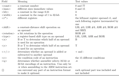
As explained earlier, we limit our focus on the core instructions of the ARM instruction set. We compiled a set of 351 encoding formats from the Encoding A1 field of each instruction description in the ARM Architecture Reference Manual for ARMv7-A and ARMv7-R [1].

[image:41.612.46.508.320.617.2]

These instruction formats contain fields for options and operands. There are too many possible options for each field to test every combination. Thus, these fields were initialized according to table 5.1. Operand numbers were cho-sen semi-arbitrarily, based on the values allowed among all different instructions taking such an operand field. For each instruction format, each possible combi-nation of field values was created and measured.

Table 5.1: Instruction operand fields and tested values

Field Meaning Test values

<const> a constant number 0 and 77

<imm> different sizes immediate values 0 and 15

<lsb> a constant in the range 0-31 3

<width> a constant in the range of 1 to 32-lsb 8

<r*> different registers the leftmost register operand r1, and each following register incremented by one

<shift> a constant-distance shift operation on LSL #3, LSR #3, ASR #3, ROR #3

an operand and RRX

<rotation> a bit rotations in the operation ROR #8

<type> a register-based shift type on an operand LSL, LSR, ASR and ROR

<x> B or T to determine which half of an operand B is used for an operation

<y> B or T to determine which half of an operand T is used for an operation

<+/-> determines whether an operand is added or + and -subtracted to another operand

<c> the condition code of an instruction the 15 different conditions

<q> determines whether assembler selects 16-bit or .w 32-bit encodings of an instruction. Can only be .w when assembling to the ARM instruction set.

{} can surround any part of an instruction format each optional part was included and

to make it optional. not included

Instructions using the fields<spec reg>,<endian specifier>, and<option>

(42)

5.5 Methodology

The timing model is constructed by measuring issue time and latency of executed instructions. The instructions are executed in different contexts, to measure the effects and existence of the influences described in section 5.2. To filter out noise, instructions are executed multiple times – typically 512 to 2048 times – and the measured time is divided by that factor. This process is repeated multiple times for each instruction and the quickest execution time is regarded least noisy. This approach leads to results which are over-approximated by no more than a twentieth of a cycle, which we explain by noise and overhead from the cycle-measuring function calls. The results are rounded down to compensate for this over-approximation.

5.5.1 Initial Measurements

A first indication of issue time is acquired by consecutively executing the same instruction. Execution time does not depend on availability of registers, because different registers are used for all source and destination operands. This setup thus measures issue time. However, this setup does not take into account any instruction optimizations which influence execution time by specific instruction interactions. Specifically, this measurement leads to false results for instructions which can dual-issue as younger. Because all instructions which can dual-issue as younger can also dual-issue as older, all such instructions dual-issue and are thus measured at half the actual execution time. However, since all instruc-tions which can dual-issue have an issue time of 1 cycle, all instrucinstruc-tions which can dual-issue as younger are known after the initial measurement because the measurements say they take up 0.5 cycles.

5.5.2 Dual-Issue as Older Instructions

(43)

5.5. METHODOLOGY 35

5.5.3 Latency

For the following measurement setups, we refer toknown-timing instructionsby which we interleave instructions we measure. The chosen instructions do not matter specifically, as long as they are not affected by optimizations in specific combinations of instructions. The problem with our measurement setup is that we must rely on machine instructions, to measure other machine instructions. Thus, if we have an incomplete understanding of the instructions supporting the setup, this can negatively influence our understanding of other instructions. Based on trial-and-error, we assume that the issue time of the multiplication instruction MUL is not influenced by any specific instructions executed before it. If such behavior is unknown, consistency of results needs to be validated in hindsight. We have not found any evidence that disproves this assumption.

Because instruction issue time is known from previous instructions, latency can be determined by interleaving the tested instructions with a known-timing instruction which takes an output operand of the measured instruction as an input operand. A naive approach is to feed the output from the tested instruc-tions into the input from the following tested instrucinstruc-tions. However, this does not take into account timing influences of the input operands, such as early and late operands. However, by interleaving the instructions with a known-timing instruction, the measurements are performed under the same conditions for all instructions.

Again, the execution time of the interleaved instructions needs to be sub-tracted to compute the latency. Because the interleaved instructions depend on the tested instruction’s output, the latency of the instruction is measured. Not all instructions have output operands, so latency does not apply to these instructions. In our measurement results, this demonstrated as measured timed being equal to the instruction’s issue time.

5.5.4 Early and Late Operands

To measure which instructions take early and late operands, the setup for mea-suring latency is reversed. In this setup, theinput of the measured instructions depend on theoutput of interleaved known-timing instructions. Taking into ac-count the interleaved instructions, computing the difference between the mea-sured time and the time meamea-sured under normal conditions reveals how much earlier or later operands are required.

5.5.5 Bypasses

(44)

i.e., an instruction of which it is known that it can bypass its result, was inter-leaved by instructions which took the bypassing instruction’s output as input.

5.5.6 Condition Codes

To measure the effect of condition codes, two measurements were performed for each condition code. For the first measurement, the flags are set so the condition is unsatisfied, and the measured instruction thus does not execute. For the second measurement, the flags are set so that the condition is satisfied, and the instruction does execute. The execution time of these instructions was first measured separately so that this overhead could be subtracted from the measurements.

5.5.7 Memory Instructions

For the measurements of other instructions, operand fields were chosen without considering the instruction result. However, our setup demands that memory instructions receive more attention. Because our measurement setup is located in user space of a general purpose operation system, we cannot access arbitrary memory locations. However, even if our code was run on the hardware directly, writing to arbitrary memory locations could overwrite the measurement code, and arbitrary memory accesses are thus inadvisable.

To compensate for this, memory addresses were not arbitrarily constructed from the field values of table 5.1. Instead, all memory accessing instructions had their addresses computed relative to the stack pointer, i.e., we claimed a block of multiple bytes on the stack and used their location for our accesses. Furthermore, the multiple store and multiple load instructions were tested with different size register lists.

5.5.8 Branch Instructions

A special setup was required to test branch instructions for two reasons. Firstly, the branch-predictor influences execution time of some branch instructions. Sec-ondly, branch instructions directly influence the executed program paths, thus they can also influence the measurement logic. Therefore, extra logic is required to jump to valid locations and still allow for meaningful measurements of the instructions. Branch instructions were measured in a loop in which they could jump to an address later in the same loop.

Cycle Accurate Timing Channel Analysis of Binary Code