An algorithm for scheduling containers on barges

AN ALGORITHM FOR

SCHEDULING CONTAINERS

ON BARGES

public version

An algorithm for scheduling containers on barges

Author: Simon Pruijn

s1598937

[email protected]

Supervisor University of Twente: Dr. Ir. M.R.K. Mes

Supervisor NexusZ: MSc. M. Glandrup

EXECUTIVE SUMMARY

INTRODUCTION

Multimodal Container Service (MCS) transports containers using barges between five inland

terminals and the Port of Rotterdam. Currently, human planners at MCS need to manually decide which container gets assigned to which barge. Each barge sails according to a prede-termined fixed schedule between one of these five inland terminals and the Port of Rotter-dam. The Port of Rotterdam contains multiple terminals. It differs every time which termi-nals are visited to load and unload containers within the Port of Rotterdam.

The current schedules are not optimal, meaning that the barges could move more efficiently. Human planners could benefit from a decision support system. Currently, no scheduling al-gorithm is available to provide the planners at MCS decision support. In this research we therefore solve the core problem “Planners have insufficient decision support” by designing an algorithm and proof of concept to provide the planners at MCS better decision support.

APPROACH

To design our own algorithm, we conducted a literature review, performed a data-analysis, held interviews and used our own expertise.

In the data-analysis we found the following:

1) Large discrepancies exist for the number of containers loaded and unloaded; both within and between terminals.

2) Barges arrive on average 5 hours and 17 minutes earlier at the terminal than they are planned to.

3) Handling time can be forecasted in a linear model with a constant initialization time of 15 minutes and 48 seconds and a variable time of 2 minutes and 26 seconds per container.

The current scheduling process consists of four steps: 1) Use date provided by customer

2) Choose feasible modality

3) Make sure capacity is not exceeded 4) Optimise schedule

Whereby the quality of step 4 depends upon the quality of the human planner and differs largely.

THE ALGORITHM

In our algorithm, the sail schedules between the inland terminal and the Port of Rotterdam are a hard constraint and therefore always preserved. Also, the capacity of the barge is used as a constraint. For our algorithm we define the following five steps:

1) Generating priority matrices 2) Filling the barge

3) Repeat step one and two for the next voyage 4) Optimize the schedule

5) Sequencing

makes it hard to draw a decisive conclusion on the performance of step 1 and 2 of our proof of concept.

When comparing the sequences generated in step 5, we found that planners visit inlets in another, better, order than assumed for the development of step 5. This can easily be imple-mented by changing the order of the terminals in the list of step 5. Furthermore, we saw that human planners take small numbers of import containers if a barge is already nearby. This can be implemented by adding a rule that allows for earlier pickup of small amounts. Fur-thermore, we saw some variations with no traceable reason. In conclusion: step 5 of the algo-rithm can be valuable in decision support with the proposed improvements.

CONCLUSIONS AND RECOMMENDATIONS

With the proof of concept, we proved that a schedule can be generated that is comparable to a schedule made by human planners. However, we did not have access to the same data that is available to the human planners.

We cannot say with certainty whether the developed algorithm is good enough to be imple-mented. It should be tested in a fair test where human planners and the algorithm have the same input data. However, we did test step 5 elaborately. This step can be implemented im-mediately in the decision support tool, with the made recommendations.

The proof of concept has only been tested on a sample set of five distinct voyages between Meppel and the Port of Rotterdam. To test dependency effects, series of voyages should be tested. To test if the algorithm can also be applied to other inland terminals than Meppel. From our research the following recommendations follow:

1) It is important to research how the data integrity can be improved. To improve out-put quality, it is most important that time windows are registered correctly, and old data is removed from the main database. Furthermore, data should be validated be-fore entering the database.

PREFACE

This research contains the bachelor’s thesis “an algorithm for scheduling containers on

barges” to complete my bachelors program Industrial Engineering and Management at the

University of Twente.

I want to thank my company supervisor, Maurice Glandrup, and my supervisor at the Uni-versity of Twente, Martijn Mes, for their patience on my journey and great feedback on con-cept versions of this report. I would like to thank Jacob Boorsma, manager barge and truck planning at MCS, for the great insights he provided in the interview. Furthermore, I would like to thank Saskia Hidding for her support on writing and grammar.

You are reading the public version. For questions the author can be reached on [email protected].

Simon Pruijn

CONTENTS

Executive summary ... iii

Preface... v

List of definitions ... vii

1 Introduction ... 1

2 Systematic literature review ... 7

3 Context analysis ... 15

4 Solution design ... 29

5 Evaluation Proof of concept ... 41

6 Conclusions, recommendations and discussion ... 47

7 References ... 51

Appendix A: Lists of barges and terminals ... 53

Appendix B: Problem identification and problem cluster ... 54

Appendix C: Lists of Key Concepts ... 55

Appendix D: Search strategy literature review ... 56

Appendix E: Summary of content articles literature review ... 57

Appendix F: Interview form... 59

Appendix G: Analysis waiting times, handling times and difference actual time and planned time ... 60

Appendix H: Regression ... 62

Appendix I: Epoch times ... 66

Appendix J: Input list for terminal sequencing ... 67

Appendix K: Comparison of the algorithms ...68

Appendix L: Schedule sequence comparison ... 73

Appendix M: Step 5 sequence comparison ... 78

LIST OF DEFINITIONS

Barge Ship used for transporting containers at inland waterways.

Call An order of a customer containing information about how many con-tainers should be shipped at a certain moment from point A to B. Handling Time The time a barge is placed under the crane up until the barge leaves

the terminal. In this time containers are loaded and unloaded. Heuristic A rule or set of rules to find a solution to a problem. A heuristic is an

approach to solve the problem with a practical methodology, but does not guarantee to find the optimal solution.

Median The middle value in a row of values. If the amount of data in the sam-ple set is an even number, the median is the average of the middle two values. For example, in the dataset {2, 2, 4, 5, 12}, 4 represents the median.

Mean The mean is the average value of a sample set. In the case of the sam-ple set {2, 2, 4, 5, 12}, the mean is (2 + 2 + 4 + 5 + 12) / 5 = 5.

Modality 1.Way of transportation, e.g. barge, truck or train.

2. Software MCS uses to register calls and corresponding data. NLink Name of the web interface containing information about containers,

barges and schedules for the voyages containers make.

onTerminal Name of the digital field containing the time at which an export con-tainer should be delivered or an import concon-tainer should be picked up. Planner Person who schedules the containers.

Planning (verb) Long term assignment of resources.

Offline planning The planning that takes place before a vehicle has started the motion (Shiller, 2015).

Online planning Planning that takes place after a vehicle has started its motion (Shiller, 2015).

Scheduling The process of determining the sequential order of activities, assigning planned duration and determining the start and finish times of each activity.

Terminal A place where containers are loaded, unloaded and stored.

TEU Twenty-feet Equivalent Unit, the size of a container with a length of 20 feet.

Time Window Defined period of time in which an action can happen. For example the pick-up of delivery of a container.

VBA Abbreviation for Visual Basics for Applications. A programming lan-guage developed by Microsoft to be able to program macros for pro-grams such as Excel.

Vessel Ship used for carrying freight on sea. Opposed to a barge, which is used for inland transport, a vessel is used for intercontinental transport.

Voyage Trip of a barge from an inland terminal to the Port of Rotterdam (also called export voyage) or trip of a barge from the Port of Rotterdam to an inland terminal (also called import voyage).

1

INTRODUCTION

In this chapter we introduce the problems with scheduling containers on barges. First, we explain the current situation in Section 1.1 in a qualitative way. In Section 1.3 we name our core problem and explain the path towards solving it. In Section 1.4 we name the means and currently available material for this research. To conclude in Section 1.5 we lay out the re-search objective, rere-search questions and approach, providing a road map for this rere-search and an overview of the questions per chapter.

1.1

CURRENT SITUATION

This assignment is commissioned by NexusZ, a company that makes client-driven software for transport companies. One of the companies that uses the software of NexusZ is

Multi-modal Container Service (MCS). MCS calls itself Full Service, meaning that they provide the

entire routing solution between the Port of Rotterdam and the customer and decide them-selves what vehicles they use for transport, while respecting the customer's wishes. MCS uses trucks and barges to transport containers. Large parts of the planning process are done manually by five human planners who take care of the customers’ wishes.

To delimit this bachelor assignment, the scope is limited to barge planning. A barge involves a major capital investment and the daily operating costs are high. This means that improving barge utilization can be translated into significant financial improvements. Improving barge utilization also means that there are less barge voyages or less trucks needed to ship all the containers. This potential reduction in transport operations can reduce the damage to the environment.

MCS transports, according to their website, around 100,000 containers per year. MCS uses barges to ship these containers between Meppel, Groningen (Westerbroek), Leeuwarden, Harlingen, Kampen and Rotterdam. The assignment of these containers to barges is done by the human planners. Currently, NexusZ is designing a web interface named NLink to provide an overview and support decision making. Based on this information the planners can decide when to ship which container on which barge. The quality of the generated schedules com-pletely relies on the experience of the planners. Every barge has a capacity of 156 TEU, which is equal to 156 20-feet containers.

Figure 1: The NLink interface

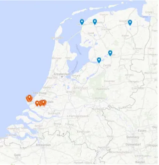
MCS uses 13 barges to transport the containers. These containers are transported between Rotterdam and the five inland terminals owned by MCS and close partners. Transportation also takes place between the several terminals within the Port of Rotterdam. A barge usually does not sail between multiple inland terminals. From the inland terminals, the freight can be transported further to the Netherlands or to other countries. Figure 2 shows the inland terminals indicated in blue and the outland terminals indicated in red. Appendix A contains two lists; one with the names of the barges and one with the terminals.

Currently, human planners need to decide which container gets assigned to which barge. They plan barges to unload and load their freight at a terminal at a specific time and assign those containers to these barges. The barges sail according to a predetermined fixed schedule between one of the inland terminals and the Port of Rotterdam. The Port of Rotterdam con-tains multiple terminals and it differs every time which terminals a barge visits within the Port of Rotterdam. The planners need to consider many aspects. For example, to pick up a container, the container should be present, and the timeframe should also match the wishes of the customer. Furthermore, there are many factors that influence the realised transporta-tion time, such as waterway congestransporta-tion, waiting times at terminals and weather conditransporta-tions. A combination of online and offline planning takes place in the planning process. Offline planning is the planning that takes place before a vehicle has started the motion, online planning is the planning while the vehicle is making its cycle (Shiller, 2015).

The current schedules are not optimal, meaning that the barges could move more efficiently. This inefficient transport includes unnecessary delays, extra resources needed, excessive truck transport and poor utilization of the resources. Currently, no scheduling algorithm is available to provide the planners at MCS decision support.

1.2

PRACTICAL INFORMATION

In this section we explain various concepts that are important throughout this document. One of the concepts used in this research is voyage. With voyage an import or an export voy-age can be meant, or a combination of those. An import voyvoy-age is a barge sailing from the Port of Rotterdam towards the inland terminal for importing containers. An export voyage is a barge sailing from the inland terminal towards the Port of Rotterdam for exporting con-tainers. Each has a voyage code containing an indication for the inland terminal, an indica-tion for importing or exporting and the date the barge enters or leaves the inland terminal. A customer can order a single trip or a round trip. A round trip means that the emptied con-tainer is also returned to the terminal it was picked up. A round trip is double the costs of a single trip and is put separately into the database. Therefore, we do not distinguish between round trips and single trips in this research and treat everything as a single trip.

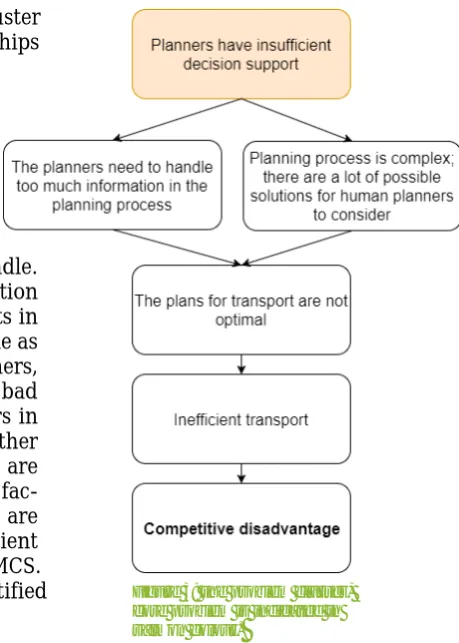
Figure 3: the problem cluster, core problem is indicated in salmon colour.

1.3

PROBLEM DISCRIPTION

A company can have several problems. A problem cluster is a helpful tool to map problems and their relationships (Heerkens and Van Winden, 2012).

At MCS the planning process does not have a de-cision support system that can generate schedules automatically. The planning pro-cess is complex. Many possible solutions and much information can be used in the plan-ning process. At this moment, more

infor-mation is available than human planners can handle. There is a trend that the availability of cargo information goes to Just in Time (JIT). There are also more aspects in cargo and infrastructure to consider than before, online as well as offline. Aspects to consider are, amongst others, the congestion on waterways, vessels that are too late, bad weather that prohibits a smooth handing of containers in the harbour, strikes, a vessel that decides to go to another harbour and reserved timeslots on terminals which are changed. Since humans cannot incorporate all these fac-tors within reasonable time, the plans for transport are not optimal, which means that there is inefficient transport, leading to a competitive disadvantage for MCS. Appendix B contains a list with all the problems identified for the construction of the problem cluster.

Figure 3 shows the problem cluster, which is mainly drawn up in consultation with the com-pany supervisor and university supervisor. As derivable from Figure 3, the core problem is defined as follows:

“Planners have insufficient decision support.”

A decision support system can support planners in doing their tasks. It can calculate many possible solutions and can take a lot of information into account while doing that. Therefore, the main question of this research is:

“In what way can planners use decision support and to what performances can this lead?”

1.4

MEANS AND CURRENTLY AVAILABLE MATERIAL

Several means are available to complete this research successfully. One of the means is the current software NLink, which has a test account to see how the software works and how the available data is interfaced towards the planners. Besides, every hour an Excel sheet is gen-erated with the current schedule containing all information that is available at that moment in the system, including, but not exclusively, the voyage number, terminals, times wished by the customers, and planned times. The system also generates an Excel sheet with the current orders on an hourly basis. These sheets provide insights in how human planners plan and think, since every hour a new sheet is generated. Furthermore, the Excel sheets can be used to build and test algorithms of which the logic can be implemented in NLink.

The optimal solution would be one that provides an integrated solution with the current web interface that provides useful information and is able to provide planning proposals. Howev-er, due to the time constraint, this projects’ prototype will be programmed in Excel. Parts of the logic and algorithm can be converted later to the current web interface, since this re-search bears upon the logic behind the code and not upon the code itself.

Existing bachelor and master theses that are made earlier for NexusZ contain proposals for useful heuristics. We will identify these heuristics and analyse their strengths and weakness-es. Furthermore, it is important to look at which constraints exist in barge scheduling.

1.5

RESEARCH OBJECTIVE AND QUESTIONS, KNOWLEDGE PROBLEM AND

AP-PROACH

As we recall from Section 1.3, the main question in this research concerns: “In what way can

planners use decision support and to what performances can this lead?”. The current

ver-sion of NLink already offers a lot of data and data visualisation. Therefore, to solve the core problem “Planners have insufficient decision support”, we develop an algorithm that helps the planners in faster scheduling of containers on barges by automating (parts of) the pro-cess. We formulate the main research objective as follows:

“Design an algorithm and proof of concept to provide the planners at MCS better decision support.”

KNOWLEDGE PROBLEM

A knowledge problem is a question that needs to be answered to solve the core problem. To recall our core problem is that planners have insufficient decision support. To solve this, we are designing an algorithm and proof of concept to provide the planners at MCS better deci-sion support.

To be able to design this algorithm, a heuristic is needed. A heuristic consists of a series of steps that can be followed to generate a feasible solution. Heuristics search for a local opti-mum. This is faster than generating all possible solutions and selecting the best one. A heu-ristic does not necessarily find a global optimum. We explain optima in depth in Section 2.3. Because it would take too much time to program all possible heuristics, a selection of poten-tial interesting heuristics that can be used in an automated planning algorithm is made. The knowledge problem is formulated as the following question:

“What is a good heuristic to plan the containers on barges?”

To answer this question, the following sub questions are formulated:

• What procedure is used by planners in their manual planning? • Which heuristics are available in literature that might be applicable? • What are the strengths and weaknesses of these heuristics?

• What are the ideal conditions under which the heuristic can be applied? “Good” is a widely interpretable word. In this research question, it will be measured on the following aspects:

• Expected performance with respect to call size, number of terminals visited and lateness.

The aspects researched possibly influence each other. A heuristic that optimizes on call size would probably lead to more lateness, since it considers call size as more important than lateness. A heuristic trying to find minimal lateness, however, would probably lead to less lateness but to a higher call size. Hence a trade-off should be made between outcomes.

RESEARCH QUESTIONS

Various research questions follow from the research objective. We divide each question into sub research questions and assign those to a chapter. This division gives us the following overview of this research:

Chapter 2: What are possible solutions for the barge scheduling problem that can be found in literature?

2.1 What are key theoretical concepts within barge scheduling?

2.2 Which of these concepts are applicable to the container scheduling problem at MCS?

We answer these questions by performing a literature study and studying theses in the same research field.

Chapter 3: How can an automated scheduling algorithm contribute to better decision support at MCS?

3.1 How are schedules currently made and what steps are taken? 3.2 At what points in the process are decisions made?

3.3 What output should the solution provide? 3.4 Which requirements should the solution fulfil?

We answer these questions by gaining knowledge from literature and interviews at MCS and NexusZ.

Chapter 4: How should the automated scheduling algorithm work? 4.1 Which approach can be used to come to the desired output?

4.2 Which simplifications and assumptions need to be made? 4.3 What should the model look like?

Based on knowledge gained from literature and interviews at MCS and NexusZ, we design a suitable scheduling algorithm.

Chapter 5: What performance can be expected when implementing the algorithm?

5.1 How can we test whether the developed algorithm generates an acceptable solu-tion?

5.2 What are the advantages and disadvantages of the developed algorithm?

2

SYSTEMATIC LITERATURE REVIEW

This chapter contains a systematic literature review. A systematic literature review is a scien-tific repeatable way of gaining knowledge on previous research. As stated in Section 1.5, we need to develop a good heuristic to be able to make an automated planning. Therefore, the knowledge question is formulated as:

“What is a good heuristic to plan the containers on barges?”

To partially provide an answer to this research question and the accompanying sub questions mentioned in Section 1.5, we identify heuristics that are available in literature that can be applied to planning containers on barges.

This chapter focuses on literature about scheduling. In Sections 2.1 to 2.3 we conduct a sys-tematic literature review. In Section 2.4 we discuss literature gathered in an unsyssys-tematic way. The following sub questions as mentioned in Section 1.5 will be answered:

• Which heuristics are available in literature that might be applicable? • What are the strengths and weaknesses of these heuristics?

• What are the ideal conditions under which the heuristic can be applied? We do this in the order or our research questions:

• What are key theoretical concepts within barge scheduling?

• Which of these concepts are applicable to the container scheduling problem at MCS? First we define the key theoretical concepts, then we search literature about these concepts and discuss how it can be applied to barge scheduling.

Section 3.2 in the next chapter provides more information about how planners work in prac-tice and what heuristics planners currently use to answer the sub question of the knowledge question: “What procedure is used by planners in their manual planning?”.

2.1

KEY THEORETICAL CONCEPTS IN BARGE SCHEDULING

To conduct a systematic literature review, it is necessary to start with defining the key theo-retical concepts. To gather general knowledge about barge planning, several articles have been consulted. For its high Field-Weighted Citation Impact of 43.69, the article of M. Chris-tiansen (2004) has been consulted. Additionally, the master thesis of L. Baranowski (2013) contains a list with key concepts related to planning and scheduling at a company compara-ble to MCS. Furthermore, Winston (2004) has been consulted to review any missing key concepts. The terms in these lists can be found in Appendix C: Lists of Key Concepts.

The found key theoretical concepts can be grouped into categories. By looking at similar key concepts, we distinguish the following list of categories, which are relevant to this literature review:

• Scheduling • Planning

• Mathematical Programming • Mathematical Model

• Simulation

2.2

SEARCH STRATEGY

We use the database Scopus for this search. Because of the limited time available for this re-search, if more than 100 results are found, only the first 100 results will be considered while search results are sorted on highest citation rate. For the search through the database, we formulate inclusion and exclusion criteria (listed in Appendix D, Table 11).

Based on the inclusion and exclusion criteria, we generate a search protocol to search through Scopus to find literature about heuristics to schedule containers on barges. The per-formed bibliographic search is depicted in Appendix D, Table 12.

2.3

EVALUATION

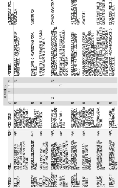
The articles found using the method described in Section 2.2 are assessed in a systematic way. Table 1 on page 9 shows an overview containing the used method, main concepts and an evaluation of each article. The main concepts are numbered, and a cross indicates that the article discusses (1) scheduling, (2) usage, (3) call size, (4) number of terminals visited and/or (5) timeliness. Furthermore, it shows the chosen performance indicators if a quanti-tative analysis has been performed in the article.

ALGORITHMS FOUND

A wide variety of algorithm types are found in this literature research. In barge planning, not one specific heuristic seems to be widely applied. Many authors use their own developed heuristics or provide a summary of research done before. Appendix E shows per article the found content. Below we provide a general overview.

Table 1: Evaluation of the literature review. (*) Concepts are numbered to save space. 1. Scheduling, 2. Usage, 3. Call size, 4. Number of terminals visited, 5. Timeliness

Local and global optima

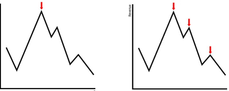
To further illustrate how the optimization techniques simulated annealing and tabu search work, a reader should first be aware of the difference in local and global optima. An optimum is the best possible result. In terms of money this often concerns the minimization of costs or the maximization of revenue. Other examples of optima applied to barge scheduling are the maximization of barge utilization or minimization of terminal visits.

A global optimum is the best of all possible solutions. In the case of revenue, the global opti-mum would be the highest peak in Figure 4. A local optiopti-mum is a point where all neighbours provide a worse output than that local optimum. A neighbour is an input of almost the same settings. In our example in Figure 4, we see that if we move slightly left or right from the red arrow, we end with a worse solution. A local optimum can be, but is not necessarily, a global optimum.

Figure 4 Left: the red arrow indicates the global maximum, Right: the red arrows indicate local optima.

Several optimization techniques exist to find the optima. Figure 5 shows the basic idea for local search methods. We start with the red arrow in the figure on the left. By moving to the left we move to higher revenue until we find a point where both neighbours are lower than the current point. By using this local search method we find a local optimum.

Figure 5 Local search method, adjusted from Krul (2016).

Simulated annealing

“The idea [of simulated annealing] is that solutions leading to a worse objective value com-pared to the current solution, should not be denied in all cases, but are sometimes accepted to find a better local optimum, or even the global optimum.”

(p. 29, Krul, 2016)

Simulated annealing has its analogic origin in the cooling of steel. Simulated annealing con-sists of two steps. First a random but feasible solution is generated. Then this solution is op-timized. This optimization is done using a so-called temperature. This temperature is high at the beginning and decreases every step. With the decrease of this temperature, also the chance of accepting a worse solution and thereby escaping a local optimum is decreased. In the beginning the acceptance probability is close to 1, while at the end the acceptance proba-bility of accepting a worse solution reaches almost 0.

A more extensive explanation on simulated annealing is given by Krul (2016).

Tabu search

Tabu search is like simulated annealing another method to escape local optima. It was intro-duced in 1986 by Fred Glover. The basic principle of tabu search is to pursue the search whenever a local optimum is encountered by allowing non-improving moves. (p. 169, Gen-dreau and Potvin, 2005)

Tabu search chooses from all its neighbours the best solution that is not the Tabu list. The tabu list contains solutions that have been evaluated previously. The choice for another tion that is not in the tabu list is made, even if this solution is worse than the current solu-tion. The algorithm can stop after a fixed number of iterations or after several iterations without improvement. The computer then takes the best solution found. A tabu search can be commonly noted in the following way (adapted from Gendreau and Potvin (2005)):

Notation:

• S the current solution,

• S* the best-known solution,

• f* value of S*,

• N(S) the neighbourhoof of S,

• Ñ(S) the ‘admissable’ subset of N(S) (i.e. non-tabu or allowed by

aspira-tion) • T tabu list.

Initialization:

Construct an initial solution S0.

Set S := S0, f*:= f(S0), T := Ø. Search:

While termination criterion not satisfied Do

select S in argmax[f(S’)]; //S’ is part of Ñ(S)

If f(S) < f* Then f* = f(S); S* = S;

record tabu for the current move T (delete oldest entry if necessary); End If

End While

EXPLANATION OF SEARCH RESULTS

In our systematic literature research, we did not find many articles about algorithms applied to barge planning or scheduling. One of the reasons therefor could be the following:

“Barge planning is originally done by employees with great naval experience, who are not open to technological advancements. With the change in the sector of coming in extra people with an academic background this seems to change, but at this point in time it seems that we are not there yet.”

(p. 13, Christiansen, 2004)

Another reason could be that this research area mainly takes place at companies where this is part of the core business. Therefore, much research into the exact algorithms and heuris-tics is confidential. Furthermore, another reason could be that we filtered on high citation rates, while applied research is cited less than abstract research.

During our research, we also found literature in an unsystematic way. In the next section we briefly discuss this literature and their relevance to our research.

2.4

SIMILAR LITERATURE IN THIS FIELD

In addition to the systematic literature review, it is important to also look at literature simi-lar to this research. This comparable literature can be applied more directly to this thesis’s field of research. In our systematic literature review we found mostly abstract concepts for algorithms, because the more abstract theories are cited more often. However, the abstract theories are hard to apply directly to our problem. Therefore, we try in this section to sup-plement the abstract theories with more applied research.

Three theses have been made for NexusZ in the near past. One of these is written by David de Meij (2014) who analyses what data can be used and what data needs to be collected for fu-ture use in barge scheduling at Combi Terminal Twente (CTT). CTT is a multimodal transport company, meaning they use barges, trucks and trains to transport containers. In this way, CTT is like MCS, with the difference that MCS does not offer transportation by train.

The thesis of De Meij does not focus on an algorithm, but focuses more on data gathering, data integrity and data visualisation. De Meij also conducted a literature study and concludes that similar problems to barge scheduling can be found in the Traveling Salesman Problem as described by Lin & Kerninghan (1973) and in the Vehicle Routing Problem as described by Christofides (1976).

Another thesis is written by Inge Krul (2015). The goal of this thesis is to “give support to the

truck planners at CTT with scheduling to improve the performance of container transport”.

Krul researched which Key Performance Indicators (KPI) are relevant in container transport. She finds the following KPIs important for customers:

Not in time

Number of containers that are not loaded at the loading/discharge time.

Time too late

Time not in time window

Lateness outside an assumed soft time window. Customers provide a hard loading/discharge time, but a certain amount of time outside this hard time provided by customers is consid-ered as on time in this KPI.

Not in time window

Total number of containers delivered outside the soft time window. No distinction is made between 2 minutes or 2 hours too late.

Krul considers the following KPI’s to be important for transport companies:

- Total number of trucks

- Travel time

- Waiting time

- Number of detours (moves where a truck does not transport a container)

- Total time of detours

Krul develops in the Plant Simulation software from Siemens a simulation model to test sev-eral experimental factors, under which the start- and stop temperatures and cooling factors for simulated annealing. She also experiments with the probability of choosing an operator (crossing, moving, or swapping a depot) and with the number of jobs that are swapped or moved with that operator.

The thesis of Lina Baranowski (2013) introduces a model that assigns containers to barges in a priority-based system. She prioritizes barges based on how many days in the time window are left and whether the barge is entering or leaving the Port of Rotterdam. Then she propos-es several filters and different ways of assigning containers to bargpropos-es. Since she found the filter containing a priority and distance-based algorithm performed best, we will focus on that approach. The problem Baranowski solves with this algorithm shows many similarities with the problem described in this thesis. However, the model she built contains an objective function containing only the minimization of late arrivals and pickups, while we also want to optimize upon other factors. Furthermore, she formulated her priorities in terms of days, making it harder to apply to voyages with irregular intervals. In our algorithm design we de-velop an algorithm dealing with these weaknesses.

All theses mentioned in this section are publicly available to read at http://essay.utwente.nl.

2.5

CONCLUSION

The goal of this literature research chapter was to find an answer to the following question:

“What are possible solutions for the barge scheduling problem that can be found in litera-ture?”

Several construction heuristics are available. The most relevant construction heuristic we found in literature is an insertion heuristic. This heuristics’ strength is that it provides a fea-sible result in a reasonable amount of time. However, the weakness is that the result is not proven to be (close to) optimal, so therefore it is advisable to use it in combination with an improvement heuristic. The classical case to apply this heuristic is in truck-routing problems without very narrow time windows, so it is debatable how useful this heuristic is in the barge planning problem.

We also evaluated three former written theses. In these theses we found that L. Baranowski developed a priority-based algorithm. We use this algorithm as inspiration in Chapter 4 at developing our algorithm.

3

CONTEXT ANALYSIS

In this chapter we answer the question How can an automated scheduling algorithm

con-tribute to better decision support at MCS? To provide an overview of how barge scheduling

works, several interviews have taken place with the company supervisor at NexusZ and the manager barge and truck planning at MCS. The structured interview form at MCS (in Dutch) can be found in Appendix F.

First, we look at the quantitative aspect of scheduling containers on barges. We analyse data gathered over several months, to gain insights in container amounts, waiting times and han-dling times. In the second part of this chapter we look qualitatively at how human planners currently come up with a feasible schedule.

Note: in the public version some terminal names, tables and graphs have been censored. The terminal names are censored per paragraph, and do not have a common letter.

3.1

DATA ANALYSIS

In this section we perform a quantitative analysis upon data from the database. First, we look at averages and spread for the containers per terminal for each voyage, then we want to know more about the number of containers per day, and finally we analyse waiting and han-dling times at terminals.

CONTAINERS PER TERMINAL

To analyse how many containers MCS transports and how they are distributed, we look at a shipper manifest Excel-sheet. This sheet contains data of actual voyages, alongside with planned times and loading and unloading amounts. We look at StartDates (the time a barge arrives at the terminal and starts the queue) between 26-09-2017 and 20-11-2017 and

Planned times between 1-10-2017 and 22-11-2017 after clean-up. These data ranges are cho-sen for the pragmatic reason that this is all data that is available at hand. In the clean-up of the sheet we removed all rows that did not have a moment registered for the actual unload or actual load time. Furthermore, all rows without a StartDate are removed. Then we created a pivot table from the data to come to the following analysis.

Table 2 shows the average number of containers that is loaded and unloaded at each termi-nal stop in a voyage. It shows the planned numbers and the actual numbers for the consid-ered period. It also shows the standard deviation and the maximum and the minimum num-bers entered in our dataset. We see that, on average, more containers are actually loaded and unloaded than planned.

Containers

Unload Planned Containers Load Planned Containers Load Actual Containers Unload Actual

Average 7.89 8.87 8.65 9.25

Standard Deviation 12.82 15.00 13.90 15.25

Maximum 106.00 137.00 124.00 137.00

Minimum 0.00 0.00 0.00 0.00

Table 3 shows the average amount of containers to unload and load which are planned, and the average amount of containers to unload and load that are actually loaded and unloaded. As we see, there are large differences between terminals. Some unload a small number of containers, such as the terminal WHT, but then load on average a relatively high number of containers. In the case of Terminal A this is 11.07. There are also terminals that are more balanced in the loading and unloading amounts, such as Terminal B.

Terminal AVG Unload Planned AVG Load Planned AVG Unload Actual AVG Load Actual

Table 3 Average Load and Unload containers per terminal

Figure 6 shows the actual numbers of loaded and unloaded containers per terminal in a graphical representation. As stated before, we see that terminals rely often heavily on either loading or unloading. Terminal C is an exception to the rule, here we see two bars of around the same length, showing that here loading and unloading is almost equal. The reason for this is that Terminal C actually covers the function of depot, meaning that containers can be delivered and picked up for storage.

Figure 6 Unloaded and Loaded actual number of containers average per voyage

CONTAINERS PER DAY

We also want to know how many containers are transported each day by barge. Table 4 shows how many containers are planned, and actually unloaded and loaded. From the data set we derive that each day around 190 containers are unloaded and 201 containers are load-ed. To readers it might seem illogical that the number of containers loaded is not equal to the number of containers unloaded. However, the dataset does not contain all containers since we removed rows with insufficient data for proper analysis. Furthermore, the dataset only covers data from a limited time horizon, which might also cause a shift. All these factors make that a difference in loading and unloading can exist.

The average of 201 containers per day is fewer than the 100,000 containers MCS states to ship yearly in Chapter 1, since 201 x 365 = 73,365. However, the dataset we considered in this chapter has been modified by removing rows with missing data. Also, the sample is from voyages planned to load and unload between 1-10-2017 and 22-11-2017. There might be a fluctuation between months that we are not able to research using this data. Furthermore, the number stated in Chapter 1 also includes containers transported by trucks, while we con-sider trucks outside the scope of this research.

Unload Planned Load Planned Unload Actual Load Actual

Total Dataset 9101 10224 9858 10448

Average per Day 175 197 190 201

Average per Voyage 80 90 86 92

Table 4 totals of containers and containers per day

HANDLING AND WAITING TIMES AT TERMINALS

To analyse waiting times, handling times and the difference between planned and actual ar-rival times, we use the same Shipper Manifest data sheet, but clean it up in a slightly differ-ent way. We define waiting time to be the time between a barge arrival and the barge is placed under a crane. In this time a barge waits for loading and unloading. We define han-dling time as the time a barge is placed under the crane up until the barge leaves the termi-nal. In this time containers are loaded and unloaded.

In Excel we filter the data by removing all rows without a crane start date (the moment the barge comes under a crane to start unloading and/or loading) and by removing all rows without an end date (the moment the barge leaves the terminal).

For this data set, the planned dates reach from 1 October 2017 to 22 November 2017. The waiting time is calculated by subtracting the start date (the time a barge arrives) from the crane start date. The handling time is calculated by subtracting the crane start date from the end date. The difference between actual time and planned time is calculated by subtracting the planned time from the start date.

If enough voyages to make a sufficiently confident analysis exist, an analysis of that terminal is made. We consider ten voyages as minimum in this analysis. For our analysis we create a pivot table containing per terminal the voyages with average waiting time, average handling time and average difference between the actual time and the planned time. The average is taken because only insignificant differences, probably due to the registration speed of the system, exist.

The analysis for each terminal can be found in Appendix G (confidential). This Appendix also provides an explanation on how to read box-and-whisker plots as we will discuss below. For readers unfamiliar with reading box-and-whisker plots, we suggest reading Appendix G be-fore continuing this section.

Figure 7a Box-and-whisker plot waiting time at BCW

Our terminal analysis shows large differences in waiting times at terminals. To compare two extreme cases: the waiting time is for 75% of the journeys at Terminal A under 10:00 minutes, while at Terminal B 75% of the waiting time lays under 3 hours and 12 minutes. The median at Terminal A is 2:08 minutes, while the median at Terminal B lays much higher at 1 hour. The box plots not only show us that there is big difference in median between termi-nals, but also in spread.

Another way to look at the waiting and handling times is by looking at the averages. For eve-ry terminal the average waiting time and the average handling time are plotted in Figure 8. We see that a large difference in average waiting times exists. For example, Terminal A offers an average waiting time of 12 minutes, but Terminal B has a waiting time of over 2 hours and

33 minutes. We also see large differences in handling time. Terminal C takes 2 hours and 10 minutes per voyage, while Terminal D has an average of 7 minutes.

However, this discrepancy in handling times can be explained by the number of containers loaded and unloaded. We only load and unload 22 containers on average at Terminal C, while we load and unload almost 70 containers at Terminal D. The handling time, therefore, seems to be largely dependent upon the number of containers.

Figure 8 Waiting and handling times of the terminals

To further investigate this phenomenon, we define a new performance indicator: the average handling time per container. The average handling time per container is defined as follows:

𝑎𝑎𝑎𝑎𝑎𝑎𝑎𝑎𝑎𝑎𝑎𝑎𝑎𝑎ℎ𝑎𝑎𝑎𝑎𝑎𝑎𝑎𝑎𝑎𝑎𝑎𝑎𝑎𝑎𝑡𝑡𝑎𝑎𝑡𝑡𝑎𝑎𝑝𝑝𝑎𝑎𝑎𝑎𝑎𝑎𝑣𝑣𝑣𝑣𝑎𝑎𝑎𝑎𝑎𝑎𝑠𝑠𝑡𝑡𝑣𝑣𝑝𝑝𝑎𝑎𝑡𝑡𝑡𝑡𝑎𝑎𝑎𝑎𝑡𝑡𝑎𝑎𝑎𝑎𝑎𝑎𝑎𝑎

𝑎𝑎𝑎𝑎𝑡𝑡𝑡𝑡𝑎𝑎𝑎𝑎𝑎𝑎𝑡𝑡𝑡𝑡𝑛𝑛𝑎𝑎𝑎𝑎𝑣𝑣𝑜𝑜𝑎𝑎𝑣𝑣𝑎𝑎𝑡𝑡𝑎𝑎𝑎𝑎𝑎𝑎𝑎𝑎𝑎𝑎𝑠𝑠𝑡𝑡𝑎𝑎𝑎𝑎𝑣𝑣𝑎𝑎𝑎𝑎𝑎𝑎𝑎𝑎+𝑎𝑎𝑎𝑎𝑡𝑡𝑡𝑡𝑎𝑎𝑎𝑎𝑎𝑎𝑡𝑡𝑡𝑡𝑛𝑛𝑎𝑎𝑎𝑎𝑣𝑣𝑜𝑜𝑎𝑎𝑣𝑣𝑎𝑎𝑡𝑡𝑎𝑎𝑎𝑎𝑎𝑎𝑎𝑎𝑎𝑎𝑠𝑠𝑎𝑎𝑣𝑣𝑎𝑎𝑎𝑎𝑎𝑎𝑎𝑎

Figure 9 on the next page shows the handling time per terminal as dark grey bars. The left y-axis depicts the handling time. The handling time per container is represented as a light grey line. The corresponding times can be found on the right y-axis. We see no correlation be-tween the total handling time and the handling time per container. People might expect that terminals with a faster handling time also have a faster handling time per container. Howev-er, we did not find a clear relation in Figure 9. The chart does suggest, howevHowev-er, that the total handling time is largely dependent on the number of containers and the handling time per container.

Waiting Time Handling Time

Figure 9 Bar and line graph of handling time and handling time per container

To further investigate this, we predict the handling time (dependent variable) with the num-ber of containers (independent variable) in the statistical analysis software SPSS using linear regression. Appendix H explicates all details on this linear regression analysis.

We can, as already suggested earlier, based on this regression analysis state that the chance of no correlation is 0%. In other words, a correlation exists. We found that the handling time can be forecasted with 2 minutes and 26 seconds per container and a constant initialization time of 15 minutes and 48 seconds.

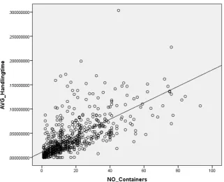
However, the data points in the scatter plot shown in Figure 10 on the next page are spread broadly from the trend line, making that predictions still contain large level of uncertainty. Also, the upper and lower bound of the 95% confidence interval for both the constant as the variable are far from the estimated values. In our analysis in Appendix H we found that 64% of the handling time can be predicted by the number of containers loaded and unloaded. To make more reliable predictions, import and export containers could be analysed individually. A model per terminal instead of one for all terminals could improve the precision too.

Handling Time Handling Time Per Container

Figure 10 correlation plot of the average handling time (in days) and the number of containers with trend line at y = 0.0016969x + .010983623

It seems that the more containers loaded and unloaded, the larger the difference between the handling time and the expected handling time. These are represented respectively by dots and the line in Figure 10.

The bar graph in Figure 11 shows the average difference between the handling time and ex-pected handling time in days on the y-axis. The difference is calculated by taking the distance of each point to the line for every sample. Then we cluster these distances in groups and cal-culate the average. We see that for groups containing less than 40 containers, this average difference is lower than 0.025 days, and for 1-10 containers even 0.012 days. For groups with more than 41 containers, this difference seems to be higher. Therefore, the model is more usable with less than 40 containers than with higher numbers.

Figure 11 Bar graph difference expected handling time and handling time

0 0.005 0.01 0.015 0.02 0.025 0.03 0.035 0.04 0.045 0.05

1-10 11-20 21-30 31-40 41-50 51-60 61-70 71-80 >81

Di

ffe

re

nc

e H

andl

ing

T

im

e

and E

xpe

ct

ed H

andl

ing

Tim

e

in

D

ay

s

Number of containers

Terminal Waiting Time Handling Time Handling Time Per

Container Planned vs Actual

Table 5 Terminals with Average Waiting Time, Average Handling Time and Difference between Planned and Actual arrival in days

Table 5 shows the average waiting time, average handling time, average handling time per container and the average difference between the time a barge was planned to arrive and the actual arrival in days. The difference between planned and actual time is negative if the arri-val date is earlier than the planned date. The difference is positive if the arriarri-val date is later than the planned date.

As we noticed earlier, high differences in average waiting and handling times at terminals exist, but not so much in handling times per container. We would expect that the barges are, on average, exactly on time in a perfect schedule. However, the average over terminals shows that barges arrive 0.22 days (5 hours and 17 minutes) earlier at the terminal than they are planned to. A possible explanation is that the planned moment is not clearly defined as whether it is the moment a barge should leave the terminal or whether, as we interpreted it, it is the moment a barge enters the terminal. Another possible explanation could be that planners like to have some extra time in their planning. The average of the difference in planned and actual times is largely influenced by Euromax. Euromax has a value of -2.10, which has some voyages with a difference in planned and actual arrival of over 4 days. This might be a registration error or a barge staying for multiple days.

3.2

BARGE SCHEDULING

Next to data analysis, it is important to look at the current scheduling method as it is per-formed currently by human planners. To improve the chances of acceptation, the algorithm should meet the wishes of the planners. Currently, barges sail at a fixed sailing schedule be-tween an inland terminal and the Port of Rotterdam, comparable to a bus line. As we recall from Section 1.1, MCS ships from and towards five inland terminals. Each inland terminal has its own sailing schedule between the inland terminal and the Port of Rotterdam. For il-lustration purposes, we show one of those inland terminals (Leeuwarden) which has the fol-lowing sail schedule:

Leeuwarden even weeks

Mo Tu We Th Fr Sa Su

Barge Barge A Barge B Barge A

Arrival 07.00h 07.00h 10.00h

Departure 15.00h 15.00h 17.00h

Table 6 sail schedule Leeuwarden even weeks

Leeuwarden odd weeks

Mo Tu We Th Fr Sa Su

Barge Barge A Barge B Barge A Barge B

Arrival 07.00h 7.00h 10.00h 10.00h

Depature 15.00h 15.00h 17.00h 18.00h

Table 7 sail schedule Leeuwarden odd weeks

Table 6 and Table 7 show the two barges that sail between Leeuwarden and Rotterdam. In the first row the days of the week are represented. Odd weeks differ from even weeks; there-fore, two tables are shown. Each barge has a time that it arrives in Leeuwarden and a time it departs from Leeuwarden.

Whereas Table 6 and Table 7 show when barges arrive at and depart from the inland termi-nal Leeuwarden, Table 8 and Table 9 show when these barges arrive at and depart from the Port of Rotterdam. In between the times in these tables, a barge is sailing between the Port of Rotterdam and Leeuwarden.

Table 8 and Table 9 show the arrival and departure times of the barges that are sailing be-tween Leeuwarden and the Port of Rotterdam. Also here a different sail schedule exists for even and odd weeks. MCS keeps distinct times a planner can schedule the barge to arrive for loading and unloading in a specific area in the Port of Rotterdam. The first time in Table 8 and Table 9 is the starting moment delivery can take place at Eemshaven, Waalhaven and Botlek. The second time is the starting moment delivery could take place at Maasvlakte I and II.

Rotterdam (From Leeuwarden) even weeks

Mo Tu We Th Fr Sa Su

Barge A Arrival in

Rotterdam 16.00 h / 21.00 h 18.00 h / 21.00 h Barge A Departure

from Rotterdam 16.00 h 7.00 h

Barge B Arrival in

Rotterdam 16.00 h / 21.00 h

Barge B Departure

from Rotterdam 15.00 h 12.00 h

Table 8 sail schedule Rotterdam (From Leeuwarden) even weeks

Rotterdam (From Leeuwarden) odd weeks

Mo Tu We Th Fr Sa Su

Barge A Arrival in

Rotterdam 16.00 h / 21.00 h 18.00 h / 21.00 h Barge A Departure

from Rotterdam 16.00 h 7.00 h

Barge B Arrival in

Rotterdam 16.00 h / 21.00 h 20.00 h / 22.00 h Barge B Departure

from Rotterdam 9.00 h 16.00 h

Table 9 sail schedule Rotterdam (From Leeuwarden) odd weeks

These sail schedules for inland terminals and the Port of Rotterdam, which are provided by MCS, are used as input for the proof of concept in Chapter 5.

CURRENT SCHEDULING METHOD

To make a schedule, orders are used which can be found in the database software. Orders arrive in various ways. Possible ways are by phone, via e-mail or in person. These orders are put via a (partly automated) system in the database software. Customers can provide a fixed date or a freely adjustable date for the containers to be picked up and/or delivered.

If an order comes in more than three weeks before it needs to be shipped, it is put into the planning system three weeks in advance. MCS has a customer policy that states that custom-ers can provide their order up to one week before the container needs to be shipped. There-fore, orders are entered into the system between one and three weeks in advance. Often in-formation on orders is still updated as time progresses. The order needs to be final the day before pickup at 16.00h.

Scheduling takes place all day. An order is moved to human planners once it is complete. The planners then add it towards a voyage. The sequence in which orders are assigned by human planners to voyages is not specified.

THE STEPS OF SCHEDULING CONTAINERS ON BARGES

If an order is complete, and it is not too early (around 3 weeks in advance) the planners can start with scheduling the order. Orders can be planned in random order. A planner focuses on one order at a time. Planners currently take the following steps when creating a schedule:

1) The planner looks at the date fields and the date range submitted by the customer. 2) Depending on the provided date range, the planner chooses whether to transport by

3) The planner makes sure that the available capacity of the vehicle at the chosen trip is not exceeded.

4) The planner optimizes the call size of the trips and number of terminals a barge visits, with the following questions in mind:

a. Can the container be switched to another incoming or outgoing voyage within the time range provided by the customer?

b. Can containers be shipped to another terminal?

c. Can the customer agree on the container being delivered outside their initially desired time range?

Some of these steps, for example 4b and 4c, require the planners to call the customers. MCS wants to try to avoid this and prefers to shuffle within the provided time ranges as much as possible. The quality at which step 4 is performed, differs largely between human planners. In practice we see that the quality of the optimization mentioned in step 4 differs between human planners. In a large part of the analysed schedules, only two or three terminals of the 25 within the Port of Rotterdam remain unvisited. In two of the five cases, a terminal was even visited twice in the same voyage. Planners also sometimes plan terminals with the same point of time, which is physically impossible to accomplish.

DECISION POINT

For the algorithm it is important to know at what point(s) in the process a decision is made. In this process one main decision is taken: a container is or is not placed on a voyage. For example, a container can be placed on voyage j and on voyage j+1. It is up to the planner to decide on which voyage the container should go. From this follows the routing. The routing depends on which containers are chosen, since this leads to a terminal being visited or not. The main point of decision in barge scheduling can also be formulated as the following ques-tion: On which trip do I take the container, where no trip is also an option? If no trip is cho-sen, the container will be transported by truck. This decision is made by the human planner in the scheduling process when orders are added to voyages.

The manager barge and truck planning at MCS sees a good decision as a decision that pre-serves the barge sail schedule as much as possible, visits the least number of terminals in Rotterdam and has the biggest possible call size. A bad decision is a decision that exceeds the date ranges provided by the customers. To improve the chances of acceptation of the algo-rithm, we incorporate these decisions as much as possible. However, sometimes it could be better to change the sail schedule if this yields lower costs, or chose to transport a container later if the fine and reputation loss do not outweigh the extra transportation costs.

3.3

THE ALGORITHM

REQUIREMENTS

To be able to automate (parts of) the process, an algorithm is needed. For a to be developed algorithm the following requirements are formulated:

2. Time windows provided by customers must be met as much as possible MCS considers time windows for picking up and delivering containers set by customers as very important, since customers expect an on-time delivery.

3. The call size must be high enough

Barges are expensive to operate. Therefore, it is important that there is a high utilization of the barge. A large call size means that there are many containers on the barge, which means that the utilization is high.

4. Where possible it must be adaptable to other companies and situations NexusZ serves many types of customers. These customers are interested in similar decision support solutions. If the algorithm is adaptable, these wishes can be fulfilled.

IMPORTANT FACTORS

Next to the requirements for the algorithm, important factors exist that the algorithm should be able to make a trade off in. The following factors are important to NexusZ and MCS:

• Preservation of barge sailing schedules • Dates and times provided by the customers • Opening times of terminals at Rotterdam

• Call size optimality: the number of containers that is being transported from terminal A to B (as high as possible)

• Number of terminals visited within the Port of Rotterdam (as low as possible to im-prove timeliness)

Using these requirements and factors, an algorithm will be developed to provide the plan-ners at MCS more decision support on the scheduling of contaiplan-ners on barges.

SOLUTION OUTPUT

The algorithm should provide a schedule for several upcoming voyages. Furthermore, deci-sion support should provide feedback on how to improve existing schedules. This indication can be given such that planners know where large benefit can be gained by contacting cus-tomers for example to ask if the time window can be changed.

3.4

CONCLUSION

In this chapter we answered the question What should an automated scheduling algorithm

be able to do? by looking at the current planning process.

We first saw in Section 3.1 that, on average, 9 containers are unloaded and 9 containers are loaded per terminal. Large differences in loading and unloading exist. We also noted that on average every day 190 containers are unloaded, and 201 containers are loaded.

In Section 3.1 we also looked at different terminals’ waiting and handling times and the dif-ference between the planning and execution. We noted that large difdif-ferences in both waiting times and in handling times between terminals exist. However, the handling time per con-tainer seems to be constant. Furthermore, we found that, on average, terminals are visited earlier than planned.

In Section 3.2 we explained that the current planning process is mainly based on the experi-ence of the planners. They work mainly based on rules of thumb. The current planning pro-cess consists of four steps:

1) Look at date field

3) Make sure capacity is not exceeded 4) Optimise schedule

4

SOLUTION DESIGN

In this chapter we look at the algorithm and what the implementation of the desired algo-rithm should look like. Recall that our research objective is to design an algoalgo-rithm and proof of concept to provide the planners at MCS better decision support. This chapter answers the question How should the automated scheduling algorithm work?

To do this, we build upon the work of L. Baranowski, since this is the most relevant applied work available in this field of research. However, the objective function Baranowski only minimizes the late arrival and late pick-up of containers. It contains no trade-off between other factors. The ideas and concepts behind her study are useful as inspiration. Therefore, we chose to use much of her work as an inspiration for our algorithm instead of using it as foundation.

This chapter is divided in two parts: the algorithm (Section 4.1) and the proof of concept (Section 4.2). In the section of the algorithm we describe a general applicable algorithm that can be applied to our case, but also to similar situations. In the section about the proof of concept we discuss our implementation of the algorithm for testing purposes to be able to value our algorithm. We end this chapter with a conclusion on both the algorithm and the proof of concept.

4.1

ALGORITHM

This section describes our developed algorithm to schedule containers on barges. It contains the approach that is used to create the algorithm. Then the steps for our developed algorithm are described. We end with the underlying assumptions for this algorithm to work.

4.1.1

APPROACH

The goal of the tool is to provide a series of schedules for the planner. Preferably, the tool should also show suggestions for improvement. Recall from Chapter 3 that a barge trans-ports via a fixed sail schedule between an inland terminal and the Port of Rotterdam; a time table like a bus line. Planners need to adhere as much to those set times as possible.

The main decision concerns which containers within the Port of Rotterdam are picked up and delivered. For the Port of Rotterdam, the planners decide which terminals are visited in which sequence and how many containers are picked up and delivered. Figure 12 shows that five separate areas or groups within the Port of Rotterdam can be distinguished. L. Bar-anowski distinguished four groups. However, the Maasvlakte II did not exist when she de-fined the areas. A barge arrives at an Arrival Day in the Port of Rotterdam and leaves at a fixed date that we call the Leave Day. In between these two dates, the barge can pick-up and deliver containers at multiple terminals. Each barge has a maximum capacity for transport-ing containers. Every terminal is part of only one group. We describe the different areas in the Port of Rotterdam by a group with a number. Group 1 contains terminals belonging to the Waalhaven, Group 2 contains terminals belonging to the Eemhaven, Group 3 contains terminals belonging to the Botlek, Group 4 contains terminals belonging to the Maasvlakte and Group 5 contains terminals belonging to the Maasvlakte II. Table 10 provides an over-view of the groups and their corresponding terminals. Figure 12 shows the location of the groups on a map of the Port of Rotterdam.

Group Terminals

1 BCW, MRS, PROGECO3, UP7, WHT

2 ITERFOR, KRAREE, MBCROT, PCSA, PROGECO, RSTNOORD, RSTZUID, UCTEEM, UCTFRISO 3 CETEM, PCTRO, WBT

4 APM, DCS, RCT, DDE, DDN, EUROMAX 5 APM2, RWG

Figure 12 grouping of terminals in Port of Rotterdam

The algorithm will focus on timeliness, since MCS appoints this as the most important factor. In the optimization step we focus on other factors which can be optimized upon, such as terminal visits or visits within the same group. However, in practice we see that the latter two seem to be of less importance to the human planners than the timeliness. In our algo-rithm, the sail schedules are a hard constraint and therefore always preserved. Also, the ca-pacity should be put in as a constraint and is therefore preserved.

For every container two options exist in the algorithm: to go with a barge today or not. If this is the last planned voyage on which a container can be transported and it is not assigned to the barge, the container is transported by truck. If this is not the last voyage a container can be shipped, it will remain in the list to be shipped with one of the next voyages.

Since new containers can come in as time progresses, it is important to schedule as many containers as early in the voyage schedules as possible. We do this by filling the barge as much towards the capacity constraint as possible. We initially do not pay too much attention to the number of terminals visited. In the optimization step (step 4), the allocation can be optimized on reducing terminal visits too.

For our algorithm we define five steps: (1) generating priority matrices, (2) filling the

barge, (3) repeat step one and two for the next voyage, (4) optimize the schedule and (5) sequencing. These five steps are further explicated below.

STEP 1 – GENERATING PRIORITY MATRICES

To be able to quickly generate a schedule, we want to transpose our lists with all container data and our barge sail schedule into a matrix. We want to create a matrix like the example in Table 11. This matrix contains for each terminal within the Port of Rotterdam the number of import or export containers, split up into priorities.

BCW PCTRO WBT APM DCS RCT EUROMAX …

priority 1 15 0 0 3 0 3 9 …

priority 2 0 0 0 1 0 4 26 …

priority 3 1 0 2 4 0 9 5 …

priority 4 13 0 1 0 0 2 7 …

Table 11 example of an unplanned import or export matrix