Evaluation of Motion Control Algorithms for Miniaturized Agents Moving Inside 3D Fluidic Microchannels

MASTER THESIS

EVALUATION OF MOTION

CONTROL ALGORITHMS

FOR MINIATURIZED

AGENTS MOVING INSIDE

3D FLUIDIC

MICROCHANNELS

Dennis Niehoff

FACULTY OF ENGINEERING TECHNOLOGY DEPARTMENT OF BIOMECHANICAL ENGINEERING EXAMINATION COMMITTEE

Prof. Dr. Sarthak Misra Federico Ongaro Dr. Ir. Ronald Aarts

Abstract

In the most recent decades, a greater focus has been put onto minimally invasive surgery which, by extrapolation of the principle, leads to microagents used in clinical applications. These agents could be injected via syringes or catheters and moved from the outside by a surgeon. Different applications for microagents are imaginable, including drug delivery to specific locations in the human body to allow for a very localized medication. A scenario for this could be the release of a drug close to a patient’s liver. Instead of injecting the drug into the blood stream and waiting for it to be transported through the whole body to all organs, a highly potent dose can be used localized instead. Harmful effects onto other organs could be reduced while potentially amplifying the effect onto the targeted region.

Realization of this, however, requires sufficiently accurate control of microagents inside of the patient’s body. The agent’s location and its drug release have to be controllable from outside of the patient’s vein system. One enabling factor for the control of microagents in 3D is position feedback which has to be provided by a clinically viable method. The imaging modality utilized in this project is ultrasound imaging. The according devices, ultrasound machines, are already widely used in medical applications, for instance to visualize the intestines of a patient or a child inside of a pregnant woman. The large accessibility of this technology in medical fields is a key factor when choosing ultrasound imaging as the imaging modality of this project.

To evaluate motion control algorithms in this project, different aspects have to be considered, the first of which is the production of suitable vein models. A convenient way of producing microchannels imitating veins had to be found to carry out any form of experiment regarding this matter. A method described in literature and an alternative new method were considered. Another aspect is the production of a exemplary drug to be transported by the microagent. Given that the produced microchannels are visually transparent, a colored substance appeared to be the most convenient solution for this. Once the substance was transported along with the microsphere, a successful release of the drug would be clearly visible if the substance was given some color. The release, in return, could only be considered successful if it could be controlled from the outside. The method chosen for this was induction heating via a magnetic field, therefore the drug to be delivered has to be sensitive to a both, magnetic fields and small fluctuations of its temperature. Imaging of the microagent is supposed to be realized via ultrasound imaging. The ultrasound probe used in this project is capable of imaging in a 2D plane. To realize continuous tracking in a 3-dimensional space, the 2D plane and subsequently the ultrasound probe have to be moved in the remaining spatial dimension. A mechanical solution for this is presented and two different approaches for the control of this mechatronic device are considered. Finally, a control structure is proposed to determine the forces to be exerted onto the microagent based on the agent’s position determined using the ultrasound tracking and a setpoint location defined by a user. The forces are supposed to be applied by a magnetic field generated outside of the vein model.

Acknowledgements

First and foremost, I would like to thank Federico Ongaro for his guidance as a daily supervisor in this graduation project. The information and insight provided by him during meetings and discussions was substantially useful for the completion of this study. Additional thanks goes to Prof. Dr. Sarthak Misra for his feedback on my progress and his support as a chairperson of my graduation committee. Next, I want to thank Dr. ir. Ronald Aarts for being the external member of my graduation committee and for the feedback that he gave.

Contents

1

Evaluation of motion control algorithms for miniaturized agents moving

inside 3D fluidic microchannels

3

I Introduction 5

II Materials 7

III Methods 10

IV Results 15

V Discussion 20

VI Conclusions 21

2

Appendices

23

A Full Derivation of the Control Structure 25

B Matlab Simulations 34

C Ultrasound Holder Design 38

Part 1

Evaluation of motion control algorithms for miniaturized agents moving

inside 3D fluidic microchannels

Dennis Niehoff

Abstract— The clinical application of drug-carrying microa-gents requires their control in 3D based on position feedback provided by imaging modalities such as ultrasound imaging. This work demonstrates the functionality of the different aspects going into the wireless control of microspheres. These in-clude production of microchannels, equipment of microspheres with adequate substances, tracking of the microagent in 3D with a 2D ultrasound probe and a proposed control structure to determine the forces to be exerted onto the microagent by an external magnetic field.

The control structure is tested in simulations and the micro-sphere is tracked initially in a steady position, then in a simple vertical microchannel and finally a curved 3D microchannel. The measurement results suggest that the developed tracking algorithm is suitable for this application and allows the setup to track the microsphere with a diameter of 1 mm inside of variable-sized, fluidic microchannels.

I. INTRODUCTION

In the year 1985, the first step has been made towards an era in which surgeries on the human body significantly changed. For the first time, minimally invasive surgery had been used to remove a gallbladder from a patient. Instead of one large cut across the human’s abdomen, only three comparably small cuts were made to allow for the surgeon’s tools to be used. More than three decades later, minimally invasive surgery can be found in nearly all different fields of surgery on the human body. The advantages of this method compared to the old procedure were so significant that there are nearly no reasons to not apply minimally invasive surgery when it is possible. Patients had far smaller wounds which in return resulted in shorter recovery times and reduced pain for the patient after the surgery. Also the chance for complications is the same as for conventional surgery or even lower [1].

The step from surgeries affecting large parts of the human body towards minimally invasive surgery had large effects on the quality of all kinds of interventions on a patient’s body. In more recent years, this idea has been taken even further: microrobots have drawn attention towards their potential applications inside of a human body. With spatial dimensions in the sub-millimeter range, these agents have the capability to move inside of human veins. The wound caused when injecting such robots into a patient’s bloodstream would not be more than a spot at which the needle of a syringe has entered the human body.

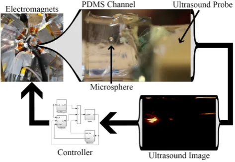
Realization of this technology however is bound to the resolution of multiple challenges [2], the first of which is the motion control of the microrobots. Commonly, robots are equipped with motors to allow for their movement in

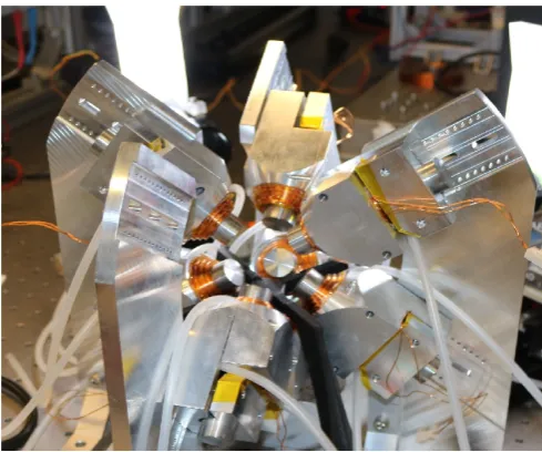
Fig. 1. Electromagnets are used to actuate the microsphere inside of a PDMS channel filled with silicone oil. The location of the microrobot is determined via an ultrasound probe which acquires according ultrasound images. These images are analyzed by a computer and the retrieved information is fed into a controller which in return determines the forces that should be applied to the microsphere via the electromagnets.

space. However, the size of the robots in this specific case prohibits the implementation of motors inside of or directly at the miniaturized agents. Even if a way was found to reduce the size of a motor to this scale, a sufficient power supply would still pose an additional challenge. Therefore, it appears far more reasonable to apply forces to the microrobots via external sources. One suitable way to apply mentioned forces are magnetic fields which could be used to effectively pull the robots through the patient’s bloodstream via electromagnetic forces acting on a magnetic part of the microrobot. A positive aspect regarding the use of magnetic fields is the fact that the human body can withstand exposure to strong magnetic fields without significant hazards [3]. The quasi-static field can pass through the human body without interacting with it, the body is effectively transparent to it.

the use of an alternating magnetic field to induce heat inside of the magnetic parts of the microrobots. Magnetic micro-particles carrying heat-sensitive materials and some form of drugs were indicated to be a potential application of this heat generation in the hyperthermic agents.

Martel et al. however also pointed out limitations of their approach [4], specifically regarding the working operating range of the setup: the magnetic fields generated by magnets have a rapidly decreasing field density with increasing dis-tance from the source of the field. Therefore, strong magnetic fields, and accordingly also large forces onto magnetic micro-agents are limited to a rather small range around the source of the magnetic field. Assuming that the magnetic field’s source was positioned immediately at the patient’s skin, it would still only allow for sufficient control within a certain depth into the human body. Larger depths could be achieved while significantly affecting the targeting efficacy [4]. Further restrictions regarding the workspace dimensions were given by the fact that Martel et al. attempted to move the particles without any actual navigation or trajectory control along pre-planned paths. Intuitively this requires the distance between the injection point and the destination to be as small as pos-sible. The paper reported that this distance had a tremendous influence on the targeting effectiveness.

With respect to the approach with the MRI scanner, the presence of rather large latencies was reported. As the MRI devices are commonly not developed for the control of magnetic devices inside of them, there are various modules involved in this particular control attempt. These modules and their interfaces add small delays which add up, caus-ing the entire communication to suffer from latencies. For eventual, elaborate control structures, these delays cause problems regarding stability and safety. Therefore, MRI scanners only offer a very limited solution to the second major challenge that has to be overcome to realize control of microrobots inside a fluidic microtunnel: The establishment of a feedback signal about the robot’s position based on some clinical imaging modality. Magnetic resonance imaging might be one solution to this problem, but it also introduces the new problem of time delays. An alternative imaging technique commonly used in medical applications is based on ultrasound.

The use of ultrasound to track microrobots has several advantages compared to MRI scanners, the first of which is the fact that ultrasounds scanning, generally speaking, is far more accessible [6]. Due to this, a direct interaction between the patient and the operating clinician is imaginable which, depending on the patient, could be very useful. Also guided operations and interventions would become possible with the use of ultrasound compared to the pre-planned paths using the MRI approach [4], [6]. Regarding the more technical aspects and especially the suitability for real-time control, ultrasound is still a good solution as it offers sufficient resolution for detection of micro-particles combined with high frame rates [7], [8], [9]. Just as magnetic resonance imagining, ultrasound technologies also have no undesirable effects on a patient’s health, but further comparison of

the two techniques shows that US applications additionally tend to be quite cost-efficient compared to MRI scans [2]. Consequently, ultrasound based feedback can therefore be regarded as a suitable solution for the second challenge regarding the realization of the control of microrobots inside of fluidic microchannels.

The third and final challenge that has to be overcome in order to allow for realization of the control of microrobots inside of a patients body, is the system’s ability to deal with the different conditions and properties surrounding the microrobots. This refers for instance to the density, viscosity and flow velocity of the medium inside of the microchannels. The system should also be able to be adaptive regarding time-variances of these properties. Furthermore, fluids inside of channels are generally strongly influenced by the presence of surrounding walls. The flow rate of liquids close to the channel walls deviates greatly from the flow rate in the center of a channel. Such surface effects should not pose a problem for the system and its control [2]. The design of a control structure which can deal with uncertainties in the system and with time-varying conditions therefore is crucial to the realization of this technology, however, the creation of such a control structure simultaneously poses a solution to this challenge.

The main goal of this project was to develop a method to control the motion of a microsphere inside of a fluidic microchannel. As a part of this main goal, it was also desired to produce such microchannels and to fill them with a fluid that has optical properties similar to the material making up the microchannel walls. The reason for this lies in the fact that similar optical properties of the surrounding and the liquid enhance the performance of the ultrasound imaging procedure that was supposed to be utilized in this study. Additionally it was anticipated to use transparent substances to allow for visual approval of the information collected by the ultrasound system. It was attempted to find a suitable coating for the microrobot such that this surrounding material could be molten via induction heating. Finally, it was a goal to realize this control by tracking the microrobot in 3D space using a 2D ultrasound imaging probe.

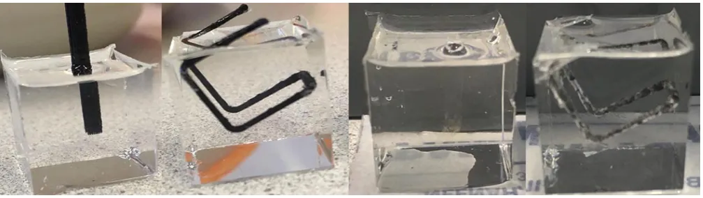
Fig. 2. Hardened PDMS cubes containing 3D printed paths of ABS. Fig. 3. The PDMS cubes after being treated with acetone to dissolve the ABS. The left channel has been filled with silicone oil.

II. MATERIALS

To allow for the realization of the specified goal, different partial problems had to be overcome. The control of mi-crorobots inside of fluidic microchannels initially requires the production of such microchannels. Then the microrobots themselves had to be selected and prepared for their task. And additionally the surrounding of the microchannels had to be prepared, this includes a mechanism to move the ultrasound probe as well as a system to generate magnetic fields. All of these aspects will be considered in more detail in their respective subsections.

A. Production of the Microchannels

When attempting to produce any kind of structure, es-pecially regarding micro structures, there are generally two possible approaches to this: either the structure can be built up directly or some kind of negative model is initially manufactured in order to simplify the production of the final structure. When different materials are processed, one or the other approach promises to be more suitable.

In this particular application, it was found that the material surrounding the microchannels should be as transparent as possible. The reason for this lies in the fact that a system of tracking cameras should be used to verify the correct opera-tion of the ultrasound tracking. Only an optically transparent material would offer this option. Additionally, the material was supposed to have similar properties to human flesh when spectated with the help of an ultrasound technique. One suitable material for these requirements is polydimethyl-siloxane (PDMS). PDMS is optically clear, transparent to ultrasound and, in the general frame of this work and after the microchannels have been produced, inert, non-toxic and non-flammable [10].

After PDMS was selected as the material building up the surrounding of the actual microchannels, a procedure had to be found to shape the initially liquid material into an appropriate structure. A procedure developed by Saggiomo and Velders [11], [12] involves the production of a 3D printed negative which is then placed inside of liquid PDMS until the polymer hardens. Once this has happened, the

3D printed material can be dissolved with an appropriate solvent. In this project, the same approach has been taken initially. The desired shape for a microchannel has been 3D printed in acrylonitrile butadiene styrene (ABS). In this first attempt, two shapes for microchannels were considered: a straight, vertical path and a path consisting of multiple straight segments connected by corners of 90 degrees. PDMS was prepared and poured into cubic containers with an edge length of two centimeters. The black ABS pieces were fixed in location from the outside until the PDMS had hardened completely. Afterwards, the cubic containers were removed, resulting in PDMS cubes with ABS paths inside of them as can be seen in figure 2.

In a next step, the cubes were submerged in acetone which should dissolve the ABS while not interacting with the PDMS. A time period of approximately 72 hours with multiple exchanges of the acetone had passed, but the effects on the ABS paths were not significant. The straight path, which did not penetrate the PDMS cube far, was almost completely cleared. Only few remaining pieces of ABS had to be removed manually. The cornered path ,however, was only cleared to a little extent. Attempts were made to remove the remaining material with tools such as needles and tweezers. However, these attempts were not successful (Figure 3).

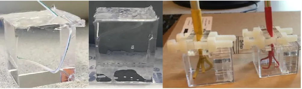
Fig. 4. Hardened PDMS cubes. The left block still contains the cable.

The right block has the cable removed and is filled with silicone oil. Fig. 5. The containers for the liquid PDMS before pouring. The cableswith bifurcations can be seen.

results of this approach were satisfying. Different cables could be used to produce channels with different diameters and the flexibility of the wire allowed for free shaping of the actual channels. Furthermore, the problem of the non-smooth surfaces was also resolves as the cables did not have steps in their surrounding electric isolation.

Due to the clear advantages of the second approach, a final set of PDMS microchannels was manufactured, also incorporating bifurcations of the channels. This was ac-complished by leading multiple cables into a straw and by sealing off the connection point with heat shrink material and with liquid glue. An indication of this is visible in figure 5. The final set of microchannels has therefore been created by placing common cables inside of PDMS and by eventually pulling them out of the hardened polymer. The channels have different diameters depending on the initial cable diameter and bifurcations and curves within the channels could be realized. The channels with widths of 1 or 2 cm have eventually been filled with silicone oil since it has very similar optical properties compared to PDMS. The final result is a PDMS cube with a volume of approximately 20_×20 _×20 mm3 _{containing microchannels filled with} silicone oil. Some remaining air inside of the microchannels formed bubbles which, due to viscous forces, did not rise through the microchannel towards the exit. Eventually, these bubbles were removed from the PDMS block by submerging the block in silicone oil and exposing them to a low-pressure environment. In this environment, the volume of the trapped air increased, allowed them to escape the channels and accordingly silicone oil could enter.

To enhance the accessibility of the PDMS cubes, an additional PDMS container has been manufactured in the development process of the samples. This container is basi-cally a rectangular hollow piece of PDMS that can be filled with silicone oil. Inside of the silicone oil, the previously addressed PDMS cubes can be submerged. This allows for imaging of the actual PDMS sample through the wall of the outer container and the contained silicone oil without loss of imaging quality and without the introduction of additional

artifacts while increasing the potential space between the ultrasound probe and the microchannel significantly.

B. Preparation of the Microrobots

The microrobots, which are supposed to be controlled in this work, also required preparation before they could be injected into the microchannels. The robots themselves are spheres with a diameter of 0.6 millimeters consisting of steel, manufactured by MiSUMi. The drug delivery of the robots should be simulated such that it is clearly visible when the transported substance is released into the surrounding liquid inside of the microchannels. Initially, colored gelatin was considered to be the simplest option for the microrobotic coating. It was however expected that problems could arise when the gelatin gets released from the microsphere into the silicone oil which fills the channels. The hydrophilic properties of gelatin would most likely prevent the colored coating from mixing with the oil. Therefore, it could have been difficult to determine if the coating actually got re-leased.

Alternatively to gelatin, coconut oil and coconut butter were considered to be better options, as they can easily mix with the silicone oil. Additionally, their melting points are only several degrees Celsius above room temperature and therefore a relatively low amount of energy is required to release the carried drugs. Since the coconut fats are colorless however, some color has to be added to them additionally.

In the coating process, the microsphere was initially heated up before being placed on some of the coating material which was solid at room temperature. The dissipated heat of the sphere allowed to shape the coating crudely around the microsphere. The coated sphere was placed inside of a freezer for approximately 5 minutes to lower its temperature and to completely solidify the coating again. Afterwards, the sphere and its load could be carefully picked up with tweezers.

It is expected that after the substance delivery, the mi-crochannels contain silicone oil mixed with the molten coating material. Cleaning of the channels is essential to re-use the same PDMS samples for further experiments. The suggested cleaning method requires to turn the contaminated microchannel upside down. The PDMS cube can be squeezed gently and some fine tool, such as a toothpick or a metal wire, can be moved inside the microchannel to allow for air to enter the channel and to reach all the way to the end of it. Repeating this process with result in an outflow of all of the colored silicone oil. Eventually the channels can be refilled with clean silicone oil.

C. Movement of the Ultrasound Probe

The ultrasound probe used in this setup was capable of imaging inside of a plane through the PDMS sample. To realize 3D imaging, the probe accordingly had to be moved in one spatial direction along the PDMS model. A tool used to achieve this, is the MiSUMi LX30 linear stage [13]. The stage comprises a linear screw shaft with a slope of 10 millimeters per rotation which causes a cart to travel along the stage as the shaft rotates. The shaft can be actuated via an additional motor. In this particular case, this is a DC motor (Maxon, Sachseln, Switzerland) [14] coupled with the linear stage via a gear head (Maxon, Sachseln, Switzerland) [15] with a transmission ratio of57_/13. The motor position is read out with the help of an encoder (Faulhaber, Sch¨onaich, Germany) [16] with 500 pulses per revolution.

From the 500 pulses per revolution, resulting in 2000 counts per revolution, and the transmission ratio of 57_/13 between the motor and the stage, it can be deduced that the whole setup has about 8769 counts per revolution of the screw shaft. Consideration of the shaft’s slope shows that one count of the encoder is equivalent to approximately 1.14 micrometers of linear motion of the cart attached to the linear stage. The control of the DC motor and accordingly also of the cart on the stage is realized by using one Elmo Whistle servo drive [17].

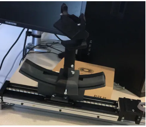
Once the stage itself was setup, it was possible to attach a 3D printed holder for an ultrasound probe as it can be seen in figure 6. This holder allows for adjustments of the ultrasound probe’s position and orientation in three degrees of freedom. Via the screws in the holder, the current configuration can be locked and the only remaining degree of freedom, translation ialong the screw shaft, is controlled via the linear stage and subsequently via the DC motor. More information regarding the 3D printed parts can be seen in Appendix C.

Fig. 6. The linear stage with the ultrasound holder attached to it. Adjustments of the probe’s orientation and location are possible via the screws in the holder.

D. Magnetic Field Generation

Another crucial part of the electromagnetic actuation of microrobots is the generation of such an electromagnetic field. Due to safety-related reasons, no permanent magnets are used to generate the field, but instead a set of coils is used as an alternative which can be shut down completely in case of an emergency. The configuration of coils used in this setup is the ”BatMag” setup introduced by Ongaro et al. [18], which consists of a total of 9 coils. The coils are powered with electric currents reaching up to multiple ampere. Accordingly heating of the coils is a factor which had to be addressed in the design of the BatMag. It has been stated in the mentioned paper that the cooling system caused the temperature of the coils to consistently remain below 120◦ _{C during the experiments that were carried out} with it. Simulations however had suggested that the coils would reach a final temperature of 700◦ _{C and that their} maximum viable temperature would be exceeded within less than 10 minutes.

Fig. 7. The setup of 9 coils used to generate the magnetic field. In the background, two cameras are positioned.

The BatMag setup has multiple properties which render it useful for the completion of this work. First off, the workspace in between the coils has an effective size of 35_×35_×35mm3 _{which is large enough to fit the PDMS} samples containing the microchannels with an approximate size of20_×20_×20mm3_{. Additionally, Ongaro et al. have} indicated that their setup was capable of levitating an iron sphere with a diameter of 1 mm. The microsphere used in this work has a diameter of only 0.6 mm and a thin coating consisting of non-magnetic substances mixed with iron powder. Therefore, it is expected that the smaller steel sphere of this work is also capable of levitating.

The two previously addressed aspects, the workspace size or workspace accessibility and the strength of the generated magnetic field however are related to one another by means of a trade-off. The setup allows for the coils to be moved further away from the center of the workspace independently, however the strongest magnetic fields can be generated in the center when the coils are closer to it. Since the ultrasound probe used for the observation of the microrobot needs to be in direct contact with the PDMS sample inside of the workspace, the electromagnetic coils cannot be moved arbitrarily close towards the center of the workspace. Instead sufficient space for the ultrasound probe and its motions in vertical direction must be provided, reducing the magnitude of the strongest operational magnetic field.

E. Ultrasound Setup

The ultrasound machine used in this setup is the Siemens Acuson S2000 [19]. It has the 18L6 HD ultrasound probe connected to it to image the PDMS samples. It is connected to a computer running Ubuntu 16.04.4 via a USB2.0 con-nection. The ultrasound machine transmits HD images at a rate of approximately 30 Hertz to the computer. The 18L6

HD probe is capable of imaging in 2D, in the plane in which the probe lies itself.

III. METHODS

Once the hardware related components of the setup were prepared, the software and control related aspects could be considered. An ultrasound probe, imaging in 2 spatial dimensions, was used to track a microrobot in 3 dimensions, hence a tracking algorithm for the ultrasound probe had to be created. Next, a computer program had to be generated to automatically cycle through the steps required for the control of the microsphere. And eventually a control structure had to be derived to determine the forces to control the microrobot in a desired way.

A. Tracking the Microsphere

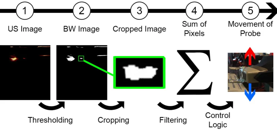
Previously the microrobots were prepared for their task inside of the fluidic microchannels. The ultrasound probe was hooked up to the ultrasound machine as indicated in section E and fixated with the linear stage from section II-C. Now a procedure had to be developed to automatically ensure that the motor in the linear stage steers the ultrasound probe towards to center of the microsphere in order to realize perfect focus. The first step required for this was to send the images from the ultrasound machine via USB-connection to a computer. The computer analyzes the image by applying a threshold criterion to the saturation of the received image. A typical example of this can be seen in figure 8 (From step 1 to step 2). The result of this thresholding is a matrix containing zeros and ones associated with high and low contrast regions in the image, indicated as black and white regions in the image. As it can be observed, there are large parts in the image which exceed the threshold limit, resulting in a white region in the processed image, even though they are clearly not associated with the microrobot. These regions are considered to be static disturbances of the ultrasound image. My means of static background subtraction, it is possible to eliminate most of these nearly constant regions such that most of the remaining white regions are associated with the actual microsphere. This improves the performance of the image tracking software significantly.

subsequently produces a matrix in which all non-zero entries refer to a pixel in the ultrasound image associated with the microsphere. Counting these pixels gives a good estimation of how well the microsphere is in focus, this is indicated as step 4 in figure 8.

As indicated earlier, the ultrasound probe is capable of imaging in the plane in which it lies. During operation, the ultrasound image will therefore always contain a circle with some radius, depending on the relative height of the probe and of the microsphere. Via straightforward geometry, it is possible to relate the observed circle radius with the imaging height of the sphere. A simplified indication of this can be found in figure 9. Assuming that ultrasound imaging on the height of the microrobot’s center would result in the observation of 1000 pixels, the observation of 750 pixels could be related to exactly two heights on the sphere, one of which is above and one of which is below the center of the sphere. Given only the maximum amount of pixels observable with a certain microsphere, it is not possible to determine which of the two heights represents reality. A way to resolve this issue would be to move the ultrasound probe into one direction relative to the microsphere and to observe the gradient of the counted pixels. Assuming for example that the ultrasound probe is located at the lower side of the sphere in figure 9 and that the probe is then moved downwards relative to the sphere - then the amount of pixels detected would decrease, revealing that the probe is located below the target height. According reasoning for the other possible cases works similarly.

For optimal control performance, the ultrasound probe

should constantly track the microsphere, preferably as close to the center of the sphere as possible. Therefore, a dis-location of the probe relative to the microrobot should be counteracted. This approach is refered to as ”tracking”. In figure 8 this is refered to as step 5. In principle there are two ways to counteract this dislocation: the first one is to make use of the maximum amount of pixels visible when the sphere is in perfect focus, the sphere’s radius and the amount of pixels counted at two locations just as described previously. With these properties, the distance from the sphere’s center is determined according to equation (1) in whichais the radius of the observed circle andris the radius of the sphere and subsequently also the radius of the largest observable circle when the sphere is in perfect focus. In principle it is therefore possible to compute the exact distance from the center of the sphere and to let the ultrasound probe move this distance in one step to exactly track the sphere’s center. The counted pixels in each configuration can be crudely related to the respective radii and the sign of the deviation is determined as in the previous example.

δ=r

r 1₋a

2

r2 (1) The alternative method to the calculation of the distance to the microsphere’s center is to move the ultrasound probe by a fixed amount disregarding the amount of pixels currently visible. If this amount is small compared to the distance computed in equation (1), the process could be repeated until the center of the microsphere is reached via this small step tracking.

Fig. 9. The amount of pixels observed for a certain relative displacement of the microsphere’s center and the ultrasound probe is not unique. Observation of a certain amount of pixels could be related to a location above and below the sphere’s center.

Both of these methods are based on a procedure that uses thresholding. Especially the edges of the observed micro-sphere are expected to cause fluctuations in the amount of pixels that are associated with the microrobot and depending on the resolution of the images analyzed, the relative or absolute amount of pixels fluctuating above and below the threshold saturation value is to be considered. The pixels, which tend to switch between black and white in step 2 and 3 of figure 8, are mainly located at the edge of the blob associated with the actual microsphere. Therefore, most of the time those pixels will be surrounded by many black pixels and only few white pixels. An attempt to counter this deviation in the counted pixels due to these alternating pixels was to only count pixels with some minimum number of white neighboring pixels. This filtering process takes into account the considered pixel itself and its 8 direct neighbors. The counting of pixels, which have a high amount of sur-rounding white pixels, effectively refers to only considering the solid center of the blob while neglecting the edge of the sphere. This results in a clearer relation between observed pixels and the relative height of the ultrasound probe and the microsphere. Depending on the resolution of the analyzed image and the pixel-threshold however, the amount of pixels associated with the microrobot may be rather low (below 40 pixels). Accordingly movements of the microsphere relative to the ultrasound probe can also only cause relatively small gradients in the amount of counted pixels. The sensitivity to small relative movements is therefore sacrificed for a less noisy signal.

An additional attempt was made to reduce the impact of the high frequency noise in the signal of the counted pixels by applying a low-pass finite impulse response filter in the form of a moving average filter. The filter length is chosen such that the noise is canceled to a sufficient degree, but that the key characteristics of the initial signal are still present in the filter output. While an increased length of the moving average filter may reduce the impact of smaller fluctuations in the signal, it also causes the output signal to follow the main trend of the input signal far more slowly.

Fig. 10. Illustration of the radar approach. In iteration 1, the probe sweeps over a wide range that includes the microsphere’s location. The position with the highest amount of pixels observed is saved and is the center of the next iteration’s sweep.

Accordingly the system’s potential to track fast movements of the microsphere is affected by this. Given that the moving average filter is computed at a rate of 30 Hz, a length of 20 would result in a filter bandwidth of 4.17 Hz and a length of 15 would result in a bandwidth of 5.57 Hz. A filter bandwidth in this region would clearly reduce the impact of the higher frequency noise compared to the rather low-frequent trend line.

Since the second method causes the ultrasound probe to carry out several small steps instead of rather large steps towards the microsphere’s center, it is far less vulnerable to noise in the input signal. A large movement of the probe into the wrong direction could result in the complete loss of focus on the microsphere whereas a small movement is expected to only reduce the amount of observed pixels by a small amount. Especially when the application is supposed to operate with a reasonably high frequency, it is therefore better to apply the second method recalling that the input signal is still non-ideal.

An alternative approach to the previously addressed track-ing of the microsphere, with one large motion towards the center or via small step tracking, is the radar approach. Instead of attempting to continuously scan a region close to the microsphere’s center, a wide range, which includes the sphere’s center, is considered. The motion of the ultrasound probe would therefore not be a set of small movements, but rather a sweeping motion with an amplitude exceeding the size of the microsphere. If these radar sweeps are located somewhere close to the microrobot’s position, then during this sweep, the microsphere must be in perfect focus at some instant of time and at some specific location. To continuously radar the microagent, the center of the sweep can be updated to this specific location. This is visualized in figure 10. The motion of the ultrasound probe could therefore be described by a sinusoidal wave with constant amplitude, but around a varying center.

the counted pixels. Even if the signal is affected by the noise to some degree, the location at which the best focus was found will not deviate a lot from the actual center of the microsphere. Crucial tunable parameters in this radar approach are the sweeping range, the sweeping frequency and the computer program’s frequency. These parameters influence to which microsphere velocities the sweeping ul-trasound probe can follow up. Since the probe is moving in a continuous upward and downward motion, its velocity has to exceed the microrobot’s maximum velocity by a factor of at least 2.

B. Program Structure

A large part of the realization of the goal in this work is the creation of a computer program that governs all the different parts involved in the control of the microrobotic agent. Based on the fact that certain parts required for the control of the microsphere were already created in C++ on Linux as a part of previous projects, this program should become a part of the already existing structure. More information regarding this structure is presented in Appendix D. Due to the existing code making use of the Robot Operating System (short: ROS), it was possible to create new programs and to have them interact and communicate with the old parts via nodes and messages.

Since the final program structure was supposed to control the robotic system in real-time, it was decided to split the overall control operation into two parts: one part should simply run the loops based on control theory which will be discussed in more detail in section III-C and the other part should deal with signals arriving from other nodes and should process them such that the actual control node would only receive the most essential information.

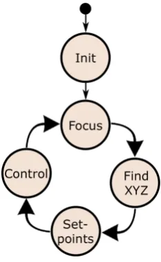
The main node has been set up such that it prepares the data from other parts of the program, which already existed previously, for the actual control node. A graphical representation of this can be found in figure 11. Firstly, the program carries out an initialization process before entering an ongoing loop. The initialization starts by setting up the ROS node of this main function and by subscribing to or by advertising certain topics to the ROS master. After the node, the subscribers and the publishers have been set up properly, the linear stage holding the ultrasound probe is moved towards its initial position. Variables for the sphere tracking process are initialized and the setpoints for the microsphere’s position are set to the current position to avoid sudden controller actions in the first program cycle.

After the initialization, the focusing process is initiated. The procedure described in section III-A is carried out to ensure that the ultrasound probe follows the microrobot and that the detected Z-position is as close to reality as possible. Via a callback incoming ultrasound images are cropped to the relevant part, pixels associated with the microsphere are counted and fed into a moving average filter. The output of the moving average filter is then used to determine whether the ultrasound probe has to move. Via the geometry of the

Fig. 11. Depiction of the program’s main structure. After initialization, the program enters a loop, focusing on the microsphere, assembling its position in Cartesian coordinates, processing potential setpoint changes and forwarding the gathered information to the control functions.

sphere, the exact position of the sphere’s center in the Z-direction is determined.

Once the focusing of the microsphere is completed, the sub-program labeled as ”Find XYZ” in figure 11 becomes active. In this part of the code, the main program receives information about the X- and Y-position of the microrobot observed with the ultrasound machine and processed by the camera tracking software. In each iteration, the distance traveled in the imaging plane compared to the previous frame is computed. If this distance exceeds a certain critical value, so that the microrobot would have traveled with an unrealistically high velocity, the program assumes that the tracking software instead has lost sight of the microrobot, focusing on some arbitrary part of the ultrasound image. The most likely cause for this event would be that the sphere focusing algorithm failed to follow up with the sphere and that the microrobot has moved entirely out of the plane of sight of the ultrasound probe. It is then possible to steer the linear stage via keyboard inputs to manually refocus onto the microsphere and to specify when the main program should return to its normal operation. During the phase in which the focus on the microagent is lost, the position vector and the setpoint vector are continuously overwritten to the last position at which the focus was not lost yet. This is done avoid random sudden controller actions as a result of a tracker malfunction and to only let the controller demand signals which cause the microsphere to stay in the position in which it got lost by the computer vision tracker. During normal operation however, simply a position vector is assembled from the X- and Y-position provided by the computer vision tracker and the Z-positioned during the focusing process.

send commands whenever it detects certain key strokes on the keyboard. These keys are presented in table I. The setpoint changes in the X- and Y-coordinates can be triggered by making use of the number block on a typical computer keyboard. To keep a certain level of overview on the key-board for a user, the setpoint changes in the Z-direction were not bound to other keys on the number block, but instead to the letters S and W. Upon occurance of either of these events, the according setpoint is increased or decreased by a fixed value of 50µm.

TABLE I

KEYBOARD INPUTS AND THEIR ACCORDING EFFECT ON THE SETPOINTS.

Input Key Setpoint Change

6 X+ ∆X

4 X−∆X

8 Y + ∆Y

2 Y −∆Y

W Z+ ∆Z

S Z−∆Z

After the current position of the microsphere and the setpoints for its position are determined, this assembled information is published to the actual control node which determines the according controller outputs. The loop of the main node then focuses the ultrasound probe attached to the linear stage back onto the microsphere and keeps repeating the same process until the whole application is shut down either by the user or by an emergency event.

C. Control Structure

According to Ongaro et al [18], the dynamics of a micro-sphere actuated by electromagnetic forces inside of a fluidic microchannel can be described as

Fem+Fd+Fi+Fg+Fb = 0 (2)

In this equation,Fem are the electromagnetic forces,Fd

are drag forces, Fi are inertial forces, Fg are gravitational

forces andFb are buoyancy forces. For either of these force

terms, it holds that F_∈R3_{. These forces can be described} according to the following relations:

Fem=∇(B·m)

Fd=−1

2ρmCDAv

Fi=Ma

Fg=Mg

Fb=−gV ρm

(3)

It can be seen from these equations that the degrees of free-dom of the microsphere are independent from one another and can therefore be considered independently. Insertion of the above relations into equation (2) allows to rewrite the system in the form of a linear second order state space system as in equation (4).

˙ xi ¨ xi = _{0 1}

0 ₋ρmCDA 2M xi ˙ xi + 0 −1 M

Fem,i+

0 −1 M di (4)

The termdin this equation is described by equation (5).

d= ∆Fd+Fg+Fb

= ∆Fd+g(M −V ρm)

(5)

In equation (4), xi indicates the position of the

micro-sphere in degree of freedom i. ρm, Cd, A and M are the

microsphere’s mass density, drag coefficient, cross sectional area and mass, respectively. Fem,i is the electromagnetic

force acting onto the microsphere in the respective degree of freedom anddiare the disturbances influencing it. According

to equation (5), the gravitational forces and buoyancy forces are considered to be disturbances as they have a constant value in each respective direction. Additionally, it is con-sidered that the description of the drag forces is not ideal. Therefore, inaccuracies in the drag forces∆Fd are included

here as well. A full derivation of this model can be found in Appendix A.1.

The reachability matrix of the state-space system in equa-tion (4) has a rank of 2 and is therefore full rank. Accordingly the system is completely reachable and the dynamics of the closed loop system with state feedback control can be described completely by the eigenvalues of the matrix A−BKwithKas state-feedback matrix. This matrix can be computed using different methods, for instance by applying Ackermann’s formula as described by Astr¨om [20]. A full example of this is included in Appendix A.2.

To enhance the performance of state-feedback control further, a feedforward component is added to the control structure. For the plant in equation (4), the control law in equation (6) is used. It follows from rearrangement of the system’s matrices. It’s derivation is worked out in Appendix A.3.

uF F =−Mx¨d−

ρmCDA

2 x˙d (6)

In this equation,xd is the desired position of the

micro-sphere and x˙d and x¨d are the according derivatives with

respect to time. Finally it is possible to rewrite this relation into a product of matrices as in equation (7).

uF F =xd x˙d x¨d

 

0

−ρmCDA 2 −M



 (7)

user-defined dynamics can be retrieved and the according first and second derivatives can be extracted from the left-hand side of the equation. By tuning the eigenvalues of this reference filter matrix appropriately, and by potentially limiting the velocity and acceleration via saturation limits before integrating them, undesirable overshoots of the actual plant’s position above the actual reference signal can be minimized as the plant follows the output of the second order filter which by definition will not overshoot the reference. This is considered with more detail in Appendix A.5.

˙ x ¨ x = 0 1

−p2 _2p x_x˙ + 0 p2 u (8)

Finally the disturbances described in equation (5) need to be considered in order to allow for all of the previous control components to work properly. This is done with the implementation of a Luenberger observer which is used to observe two signals in the system: the disturbance acting on the system, including gravity, buoyancy, model inaccu-racies and other disturbances, as well as the velocity of the microrobot in each degree of freedom. Astr¨om presents the Luenberger observer as [20]:

ˆ

x(k) = (I₋KC)(Axˆ(k₋1) +Bu(k₋1)) +Ky(k) (12) given that the plant’s state-space model has the following shape:



 xv((kk+ 1)+ 1)

xdist(k+ 1)

 =

Ad Bd

0 1

  xv((kk))

xdist(k)

 + Bd 0

u(k)

y=C

  xv((kk))

xdist(k)

 

(13) In equation (13),AdandBd are the time-discrete versions

of the state-space matrices in equation (4). Since it is only possible to observe the microrobot’s position as outputy, for this augmented plant it must also hold that

C=1 0 0 (14) Insertion of these augmented state-space matrices into equation (12) results in the description of the observer in equation (9). In this equation, xˆ2 and xˆ3 represent the estimates of the microrobot’s velocity and the disturbances

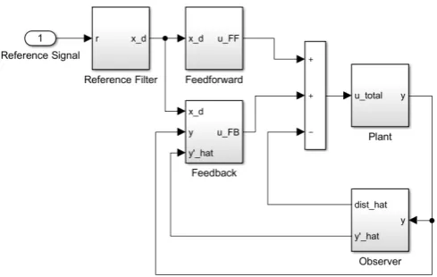
Fig. 12. Proposed control structure for the control of the microrobot including a reference filter, feedforward control, feedback control and an observer.

acting on it, respectively. The values for k2 and k3 can be computed using equations (10) and (11) which follow from the same derivation. In equations (9) to (11), aand b refer to the respective entries of the initial state-space matrices in equation (4) andprepresents the location of the observer’s poles. The full derivation of the observer can be found in Appendix A.4. A block diagram representing the final control structure can be seen in figure 12.

The control structure comprises a reference filter, feed-forward control, state-feedback control and a Luenberger observer to observe the microrobot’s velocity and the dis-turbances acting on the system. The tunable parameters are the eigenvalues of the reference filter, the state-feedback control and the observer. Given that the relation, regarding the eigenvalues of the reference filter, the feedback and the observer in equation (15) holds, satisfactory control performance is expected of the system.

pr<< pf b<< pobs (15)

IV. RESULTS

Based on the materials and methods introduced in the pre-vious sections, simulations could be carried out and test runs of parts of the setup could be accomplished. The results of these partial tests are presented in the following, a complete integration of the full setup has not been accomplished.

ˆ

x2(k) ˆ

x3(k)

=

a22−k2a12 b2−k2b1 −k3a12 1−k3b1

ˆ

x2(k−1) ˆ

x3(k−1)

+

b2−k2b1 −k3b1

u(k₋1) +

k2 k3

y(k) +

a21−k2a11 −k3a11

y(k₋1) (9)

k2=

b1p2+ (2a12b2−2a22b1)p+ (a222b1−a12a22b2−a12b2)

a12(a22b1−b1−b2) (10)

k3= −

b1p2+ 2(b1+b2−a12b2)p+ (a12b2+a12a22b2−a22b2−b1−b2) b1(a22b1−b1−b2)

A. Simulation Results

After the control structure had been derived in section III-C, simulations could be used to test whether the created structure was able to control a simulated microrobot. For the scope of this simulation, the microsphere was simulated in two spatial dimensions since the dynamics in the X- and Y-direction, the horizontal directions, are expected to be exactly the same. The additional impact of gravity and buoyancy in the vertical direction is taken into account nevertheless in this simulation. The physical properties of the simulated microsphere are documented in section IV-A.

Variable Value Description

ρm 9700 [kg/m3], density of surrounding

CD 0.5 [], drag coefficient

rmr 6·10−4 [m], radius

Amr 1.131·10−6 [m2], cross sectional area

Vmr 9.0478·10−10 [m3], volume M 4.1228·10−6 _{[kg], mass}

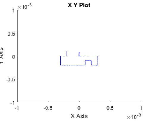
For these parameters, a state-space model has been assem-bled and discretized and according controller components have been derived with controller dynamics according to equation (15). A Simulink model has been built to simulate the effects of the controller onto the plant, additionally it was possible to change the setpoints for the horizontal and vertical simulated direction throughout the simulation. A typical output plot can be found in figure 13. In here, the simulated microagent was initially positioned in the origin of the plot. Upon increasing the setpoint in the vertical direction, in which gravity and buoyancy act, the microagent moved upwards, being traced by the blue line in the graph. The process has been repeated several times in different directions to generate the trace line in clockwise direction.

From this first simulation it appears that the controller is capable of controlling the microsphere given a perfect model of the system. To give some more weight to the capabilities

Fig. 13. XY plot resulting a simulation in which the same parameters were used for the control and for the simulation of the plant.

Fig. 14. XY plot resulting from uncertainties in the plant’s parameters and with some level of noise in the signal to the plant and from the plant.

of the controller, in a next step some uncertainties were added to the microsphere’s properties from which the controller was derived. The controller was still derived according to the entries of section IV-A, but the simulated microsphere’s properties were modified such that they deviated by up to 10% from the table’s entries. Additionally, white noise has been added to the input and output of the plant to simulate non-perfect signals in the real world. The resulting XY-Graph is visible in figure 14.

As in the previous case, the microsphere was initially located in the origin. Without any setpoint changes directed by the user, the plant moved in the vertical direction. This occurs due to the observer attempting to compensate the dynamic forces for a different plant. After approximately 0.5 seconds, the observer adjusted the error in its disturbance estimation however, allowing for normal control as in the

Fig. 16. PDMS microchannel containing a microsphere which released its coating. The microsphere was positioned at the end of the particular microchannel (red arrow), was heated with an induction heating coil and then moved away from the site (blue arrow). The leftover coating is clearly visible.

previous case. A graph of the y-position as a function of time can be seen in figure 15. In contrast to the previous, noise-free case, this time there were some small deviations from the otherwise straight movement pattern of the simulated microagent. The amplitude of these deviations was dependent on the amplitude of the noise added. More information regarding this simulation is presented in Appendix B.

B. Microsphere Coating

After a microsphere was coated with the mixture consist-ing of coconut oil, iron powder and dye, it was inserted into a PDMS microchannel filled with silicone oil. With an external permanent magnet, it was moved towards one end of a microchannel with bifurcations. The sample was placed in the operating range of an induction heating coil for 5 minutes. After the time had passed, the PDMS block was moved away from the coil and using the permanent magnet, the microsphere was navigated through the microchannel to a different loation to allow for a clear distinction between the released coating and the microsphere. The material that was transported initially by the sphere remained in the channel. An attempt of delivering the coating into the right bifurcation in figure 16, which has a small hole at the bottom to simulate a flow in the channel, had previously resulted in a yellow-orange coloring of the PDMS block as the colored silicone oil could enter the PDMS.

After the substance had spread in the microchannel, an attempt was made to clean the channel again with the method introduced earlier on. The microchannels were filled again with clean oil and eventually the channel itself was freed completely from the colored substances. This can be seen in figure 17.

C. Ultrasound Tracking

In order to test the ultrasound tracking algorithm intro-duced earlier on, one of the PDMS specimen was placed in

Fig. 17. The PDMS block that was previously used to demonstrate substance delivery after the cleaning process. Parts of the block remained colored after the cleaning because the colored oil had entered the PDMS itself.

front of the linear stage supporting the ultrasound probe. In a first step, the influence of the filtering with the moving average filter and the neighboring-pixel filter was observed. For this purpose, the ultrasound probe was fixed in a certain location relative to the microsphere inside of the fluidic microchannel such that the microrobot was in good focus. The unfiltered signal for this case is depicted in figure 19. Even though there is no relative motion of the microsphere and the ultrasound probe, high frequency deviations can be found in the signal. The same signal can be found in its filtered version in figure 20. The amplitude of the oscillations is reduced significantly, just as the frequency of the oscillation.

In the following steps, only the filtered signal of the counted pixels in each frame is considered. After the steady case was observed, the microagent was moved relative to

Fig. 19. Unfiltered signal acquired by counting the pixels in the ultrasound image associated with the microsphere in each particular frame.

the fixed ultrasound probe by means of an external magnetic field generated by a permanent magnet. An indication of this process can be seen in figure 18. Once again the microsphere was initially in good focus in its resting position. After approximately 45 seconds in the resting position, the mi-crosphere was lifted out of the focus of the ultrasound probe and the according decline in counted pixels can be observed in figure 21. Shortly afterwards the permanent magnet was moved away from the PDMS sample and the microsphere dropped back into the focus, causing the amount of counted pixels to return to its previous state. The process was repeated twice with different displacements of the microsphere, the last of which moved the sphere completely out of the focus and caused the program to pause.

After the ultrasound probe was kept in place for the previous tests, it was then instructed to move in increments of 50 micrometers while the microsphere was kept in rest. Without fine-tuning of the parameters involved in the ultra-sound tracking, a picture as in figure 22 could be observed. The left-hand side of the plot shows the amount of counted pixels while the right-hand side shows the probe’s position relative to the top position on the linear stage in millimeters. It can be clearly seen that the ultrasound probe is being moved upwards and downwards in an oscillating manner in a range of up to 0.6 millimeters. In this case the sphere’s center was located approximately in the middle of the oscillation’s extrema, around -110.3. The amount of counted pixels could support this claim, the graph showed peaks whenever the probe was moving from a low-point to a high-point and vice versa. Nevertheless the probe did not stabilize at the sphere’s center, but kept overshooting it.

With further adaptation of the adjustment step’s size and the length of the moving average filter, it was possible to minimize the oscillations around the microsphere’s center. An indication of this is visible in figure 23. In this case, the probe was initially located above the microsphere’s center and moved further towards the top edge of the

Fig. 20. The same signal as on the right-hand side after application of the filters described in section III-A.

microagent, causing the amount of counted pixels to drop. As a countermeasure, the probe was moved downwards by around 0.4 millimeters such that the probe was now located on the height of the microsphere’s bottom half. The probe was steered downwards, once again causing the amount of counted pixels to drop and eventually causing a final relatively large movement of 0.2 millimeters upwards. At this location, in between the previous two extrema, a new maximum of counted pixels was found and accordingly the probe kept this position.

Eventually, a focus was put onto continuous tracking of a moving microsphere. As the maximum velocity of the ultrasound probe in vertical direction directly depends on the distance traveled per program iteration and the amount of program iterations per second, a relatively large adjustment step size of 60 micrometers was selected. The program was running at a frequency of 30 Hz, resulting in a maximum

Fig. 22. Plot indicating the amount of counted pixels (blue) and the position of the ultrasound probe (green) in millimeters. As it can be seen, the ultrasound probe was oscillating around−110.3 where the center of the microsphere was located.

velocity of 1.8 millimeters per second. This step size left room for the oscillations about the sphere’s center once again, but also generated the results depicted in figure 24. Ini-tially the microsphere was resting in its initial position. After around 40 seconds, the microsphere was moved upwards by a distance of around 1 millimeter which can also be found in the probe’s position without a significant drop in the amount of counted pixels. The same process was initiated around 120 seconds before lifting the microsphere up by approximately 4 millimeters to the top of the PDMS sample. Fluctuations in the counted pixels could be observed without a decline of the signal below its initial level. Around 185 seconds, the observed pixels reached a local maximum associated with the relatively large fluctuations in the probe’s height. Eventually, the microsphere was allowed to drop back down to its resting position inside of the vertical microchannel. When approaching this resting position, the ultrasound probe overshot the microsphere’s location, resulting in another local minimum in the pixels.

After a simple vertical microchannel was utilized, a curved microchannel was considered next. The channel was curved, requiring the microsphere to move in all 3 spatial dimensions to traverse the channel. According measurement results are presented in figure 25. Initially the microsphere was moving mainly in the plane that the ultrasound probe was imaging. This motion was accompanied by some fluctuations about the sphere’s center while maintaining focus to a certain degree, following the microagent to a slightly higher location. Even-tually the microsphere was moved downwards by multiple millimeters through the channel which can also be observed in the probe’s position.

Finally the setup’s potential to track a microsphere inside of the additional PDMS container has been regarded. To do so, the PDMS block with the vertical path was submerged inside of the larger oil-filled PDMS container. As long as the distance between the ultrasound probe and the

microa-Fig. 23. Graph showing the amount of counted pixels (blue) and ultrasound probe’s position (green) for a stready position of the microsphere. The probe oscillated from the top end of the sphere to the bottom end before converging to the center of the sphere.

gent inside of the vertical microchannel did not exceed the ultrasound machine’s imaging depth and maximum focusing distance, the performance appeared to be identical to the op-eration of the setup when the ultrasound probe was touching the PDMS cube immediately.

D. Ultrasound Radaring

In a final test, a microsphere was positioned inside of a vertical microchannel and the program code to radar the microagent was run. The program itself was running at a frequency of 90 Hz while still receiving new ultrasound images at a rate of 30 Hz. The sweeping range was 3.8 mm and the ultrasound probe’s velocity was 5.7 mm/s. A representative output plot is presented in figure 26. In this test, the microsphere was initially in a resting position.

Fig. 25. The left plot shows the amount of counted pixels and the right plot shows the ultrasound probe’s height for a more complex, curved path. The microsphere was navigated through a microchannel in all 3 spatial dimensions. During the whole operation, the amount of observed pixels remained at a stable level.

The ultrasound probe was scanning the region around the microsphere’s initial position and there were only minor deviations in the detected sphere center of roughly 10% of the microsphere’s diameter. After 20 seconds, the mi-crosphere was moved upwards in the microchannel by an external magnet and accordingly the center of the ultrasound probe’s sweeps was corrected to a higher location as well. The microsphere was moved up all the way through the microchannel to around -83.5 mm in figure 26. In this test, the ultrasound probe could not exceed this height as it was set to be a fixed upper limit representing the top edge of the PDMS sample.

After a few seconds, the microsphere was allowed to drop down freely in the microchannel. During the whole falling process, the ultrasound probe kept track of the microagent and continued to radar it at the bottom of the microchannel. The same process was repeated a second time roughly 20 seconds later. The graph of the counted pixels in each particular frame shows several distinct spikes, each of which is associated with half of an ultrasound probe’s oscillation about the microsphere’s center.

V. DISCUSSION

A. Actuation of the Microsphere

At the start of this project, it was planned to utilize the magnetic coil setup introduced in section II-D which uses 9 coils to generate magnetic fields according to the controller structure. In general, a force in three spatial direc-tions with certain strength should be handed to a function converting this force into a set of 9 according currents. These desired currents should then be passed on to low-level CAN controllers which deliver these currents to the coils accordingly such that the magnetic field is generated to exert this particular force onto the microsphere. During the integration of the whole setup, however, it got apparent that

Fig. 26. Output plot for the radar approach. The top graph shows the amount of counted pixels and the bottom graph shows the probe’s position (blue) and the detected microsphere center (green).

the CAN controllers were malfunctioning. They were simply not providing the coils with the prescribed currents, due to faulty hardware components.

Therefore a different solution had to be found to actuate the microsphere via a magnetic field, namely actuation via a permanent magnet that is positioned at a certain distance to the microsphere such that it exerts forces with a reasonable force onto it. For testing purposes of the tracking and radar-ing approaches this was sufficient, however, full integration of the system was not possible with it since manual control of the permanent magnet did not allow for precise realization of the control signals. Additionally it was not a trivial task to continuously hold the magnet such that the desired velocity profile could be achieved. It is expected that this might have some impact on the quality of the demonstration results and that some results may have been better with actual precise control of the magnetic field.

B. Production of the Microchannels

Regarding the production of the PDMS microchannels an alternative approach to the one presented in literature has been chosen. Cables where used to rebuild a crude model of veins and to act as a core of the PDMS mold. The production process of these vein models is very simple and time efficient, but limits the potential for different shapes of channels. Additionally it is not guaranteed that the cables remain in their shape when liquid PDMS is poured onto them. The flexibility of the cables could result in bending of the vein model to some extend when adding the highly viscous PDMS to the container.