Modeling, design and characterization of a thermal flow sensor

(1)

Master Thesis

Modeling,Design and

characterization of

a thermal flow sensor

Yi Wang,BSc Supervisors dr.ir.R.J.WIEGERINK dr.ir.J.GROENESTEIJN

(2)

(3)

In this thesis, a new analytical model is introduced to predict the performance of a thermal flow sensor. The analytical model is based on the heat equations, and we add the heat-sink item into the equation, to ensure the calculation result is closer to the real performance. To verify the model, we also built a Comsol model, and the temperature profile of the analytical model is near agreement with Comsol model. Furthermore, the result of the analytical model also compares to the measuring result of the thermal flow sensor which provides by Bronkhorst.

(4)

(5)

Abstract 2

1 Introduction 9

1.1 Background and motivation . . . 9

1.2 Thesis Outline . . . 10

2 Theory and Modeling of thermal flow sensors 11 2.1 Thermal Equation . . . 11

2.2 Numerical simulations . . . 18

2.3 Thermal Equation with Different Geometry . . . 20

2.3.1 A sensor with two heaters and large gap . . . 22

2.3.2 The sensor with one heater in the middle . . . 25

2.3.3 The sensor with more heaters and different heat power . . . . 27

2.4 The Sensor with Heat-sink . . . 29

2.5 Overview . . . 36

3 Bronkhorst Sensors 37 3.1 Design . . . 37

3.1.1 The design with different diameters of channel . . . 37

3.1.2 The Sensor with Different Heater Length . . . 39

3.1.3 The design with parallel channels . . . 41

3.2 Fabrication Process . . . 42

3.3 Specific readout design . . . 45

3.4 Measurement Result . . . 47

3.4.1 Simulation and Measurement Result of Sensor with Different Diameter Channel . . . 48

3.4.2 Simulation and Measurement Result of Sensor with Different Heater Length . . . 53

3.5 The Prediction of Parameter’s Influence . . . 58

3.5.1 Distance Between Heaters . . . 58

3.5.2 Channel length . . . 59

(6)

6 CONTENTS

3.5.3 How the fabrication process influence the performance . . . . 60 3.6 Overview . . . 62

4 Conclusion and Discussion 63

5 Outlook on future work 65

Bibliography 67

Appendices

A The method to solve the constants 69

B The constant for equation 2.37 71

C The constant for equation 2.46 75

D The temperature profile of changing the distance between heaters 79

E The temperature profile of changing the distance between heaters 83

(7)

Symbol List

α Temperature coefficient 1/K

A area um2

cp Heat capacity at constant pressure kJ/(kgK)

G Heat sink’s thermal conductivity K/(W m)

Hf lat Height of the flat structure nm

Hheater Thickness of heater nm

k Thermal conductivity W/(m−1_K−1₎ kef f Effective thermal conductivity W/(m−1K−1)

L Length of beam m

Lgap Gap between heaters um

Lheater Length of heater um

ρ Density kg/(m3₎

P Power mW

Q Heat flux density W/m−3

R Resistance of heater Ω

R1 Radius of channel um

R2 Distance between center of channel and heat sink um

T Temperature ◦C

t Time s

(8)

8 CONTENTS

tchannel Thickness of of channel wall um

V Potential V

v Velocity m/s

Wchannel Diameter of the channel um

Wf lat Width of the flat structure um

Wheater Width of heater um

(9)

Introduction

1.1 Background and motivation

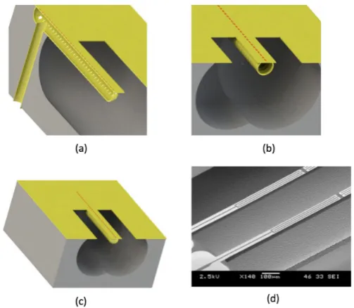
Nowadays, the thermal flow sensor is widely used in many areas, such as a drug delivery system, chemical analysis, printer, etc.. As those industries developed, the people have higher requirements for the thermal flow sensor, such as higher sensitivity, larger measurement range, and lower pressure drop. To design such a suitable sensor, we need to have an idea about how the parameters can influence the performance of the sensor. Thus we need to create a model to construct the thermal flow sensor. Usually, the researcher would like to use an FEA(finite ele-ment analysis ) software to make a thermal flow sensor model, such as Comsol [1] and ANSYS [2], the software can provide an accurate prediction of a thermal flow sensor, but the time consumption is high. Thus, in this thesis, we will introduce a new analytical model to construct the thermal flow sensor. The figure 1.1 shows the schematic of the actual sensor. The fluid will go through the closed channel via the inlet which placed in the backside of the channel, then the temperature distribution of the heater will be changed by applying the flow. Meanwhile, the resistance value of the heater embedded on the top of the channel will change, by measuring the resistance difference, we can derive the velocity of flow.

(10)

[image:10.595.158.410.87.306.2]

10 CHAPTER1. INTRODUCTION

Figure 1.1: The schematic of the actual sensor. a. Artist impressions of inlet of

the sensor. b. Artist impressions of channel of the sensor. c. Artist

impressions of the sensor. d. SEM picture of the heater.Picture takes

from [3]

1.2 Thesis Outline

Chapter 2 describes two models for the thermal flow sensor. An analytical model can be used to plot the temperature profile of the sensor in the flow direction. Later, a finite element model in Comsol is also presented to verify the analytical model/

(11)

Theory and Modeling of thermal flow

sensors

To understand the physics of the thermal flow sensor. This chapter will start by introducing the basic heat equation. Then based on the heat equation, the analytical model will be made to construct the thermal flow sensor. Also, a finite element model in Comsol will be built to verify the analytical model. Next, to make the analytical model more flexible, we will add more heaters in the analytical model. Again, a corresponding finite element model will be built to verify the results. Furthermore, based on the analytical model we made, the heat-sink will be added in the analytical model to understand how the heat-sink influence the behavior of the thermal flow sensor.

2.1 Thermal Equation

To derive the temperature profile of the thermal flow sensor, we start from the gen-eral heat equation [5]:

ρcp[

∂T ∂t + (

−

→_v _{· ∇}₎_T_{] =}_k_·_T_∇2₊_Q _(2.1)

Withρis the fluid’s density, cp is the heat capacity at constant pressure,T is the temperature, t is the time,v is the velocity, k is thermal conductivity and Q is heat

source(density).

Firstly, we assume there is no flow through the channel, and the temperature does not depend on the time, then the equation reduces to:

0 =k·T∇2₊_Q _(2.2)

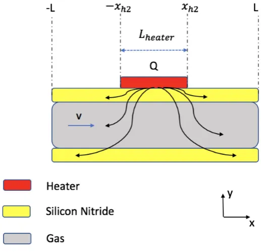
Since we only interesting the temperature profile in the flow direction, see figure

(12)

12 CHAPTER 2. THEORY ANDMODELING OF THERMAL FLOW SENSORS

2.1. Then the heat equation reduces to:

0 =kd 2_T

[image:12.595.76.477.117.372.2]

dx2 +Q (2.3)

Figure 2.1: Illustration of the how the temperature changes as applying flow. The heater placed in the middle generates the heat flow Q(donated by black arrows), and the heat flow will go through the fluid and silicon nitride. As applying the flow, the heat flux in the downstream will be larger the heat flux in the upstream. This will result in the temperature at downstream higher than the temperature upstream.

To construct the model, we need to define the geometry and boundary condition. The figure 2.2 shows the sketch of the one-dimensional model. There are is one heater in the middle, and At x = ±L the temperature will be assumed as room

temperature.According to the figure 2.2, the equation 2.3 can be divided into two equations:

0 =kd 2_T

dx2 +Q if|x| ≤xh (2.4)

0 =kd 2_T

dx2 if else (2.5)

(13)

Figure 2.2: The structure of the one-dimensional model. The heater with length2xh dissipates Q watts per cubic meter. Atx = ±Lthe silicon acts as the

(14)

T(x) =

      

A1x+B1, for−L≤x≤ −xh (2.6) −Qx2

2k +Cx+D, for|x| ≤ −xh (2.7) A2x+B2, forxh≤x≤L (2.8) With2Lis the tube length and2xh is the heater length.

To solve the equation 2.6-2.8, we need to find six equations from the bound-ary conditions. Firstly, at x = ±L the beam at room temperature, then it can be

assumed that:

T(−L) =T(L) =Troom (2.9) secondly, the temperature should be continuous atx=±xh :

Tlef t(−xh) =Theater(−xh) (2.10)

Tright(xh) =Theater(xh) (2.11) The heat flux should also be continuous atx=±xh:

[kdTlef t

dx ]x=−xh = [k

dTheater

dx ]x=−xh (2.12)

[kdTright

dx ]x=xh = [k

dTheater

dx ]x=xh (2.13)

By applying those boundary conditions into the equation 2.6-2.8, then we can get 6 equations, by solving those equations we can obtain the values forA1,B1,C,D,A2

andB2::

A1 =−A2 = Qxh

k (2.14)

C = 0 (2.15)

D= Qxh(L−

xh

2 )

k +Theatsink (2.16)

B1 =B2 =Theatsink+

QxnL

k (2.17)

If we include the velocity into the equation, the differential equation becomes:

0 =kd 2_T

dx2 −ρcpv dT

(15)

0 =kd 2_T

dx2 −ρcpv dT

dx if else (2.19)

Then the temperature at flow direction can be calculated as :

T(x) =

        

A1e

ρcpvx k +B

1, for−L≤x≤ −xh (2.20)

C1e

ρcpvx

k +C₂+

Qx

ρcpv

, for|x| ≤ −xh (2.21)

A2e

ρcpvx

k +B₂, forx_h≤x≤L (2.22)

Substituting r = ρcpv

k , and applying same boundary conditions as previously, then we have six equations as following:

A1e−rL+B1 =Troom,x=−L (2.23)

A2erL+B2 =Troom,x=L (2.24)

A1e−rxh +B1 =C1e−rxh +C2− Qxh

rk ,x=−xh (2.25) A2erxh +B2 =C1erxh +C2+

Qxh

rk ,x=xh (2.26) A1re−rxh =C1re−rxh +

Q

rk,x=−xh (2.27) A2rerxh =C1rerxh +

Q

rk,x=xh (2.28)

The equation 2.23 and 2.24 describe the temperature at the edges of the channel whichx=±L, the equation 2.25 and 2.26 describe the temperature is continuous

at x = ±xh, the last two equations decribes the heat flux at x = ±xh is also continuous. The detail about how to solve these constant can be found in appendix A, then the constant can be calculated as:

A1 =

Q(er(L+xh)₋_er(L−xh)₋₂_x

hr)

r2_k₍_erL₋_e−rL₎ (2.29)

A2 =

Q(e−r(L−xh)−_e−r(L+xh)−₂_x

hr)

r2_k₍_erL₋_e−rL₎ (2.30)

B1 =−e−rLQ(

(er(L+xh)−_er(L−xh)−₂_x

hr)

(16)

B2 =−erLQ(

(e−r(L−xh)−_e−r(L+xh)−₂_x

hr)

r2_k₍_erL₋_e−rL₎ ) (2.32)

C1 =Q(

(e−r(L−xh)−_er(L−xh)−₂_x

hr)

r2_k₍_erL₋_e−rL₎ ) (2.33)

C2 =Q(

((rxh+ 1)erL−(rxh+ 1)e−rL−erxh +e−rxh + 2xhre−rL)

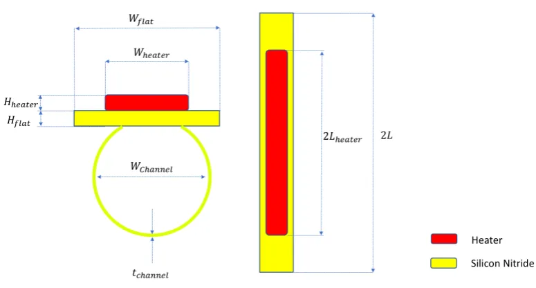
r2_k₍_erL₋_e−rL₎ ) (2.34) To construct the analytical model, we need to define the simulation parameters. The figure 2.3 provide the schematic overview of the parameters of the channel, and the table 2.1 gives the value for those parameters.

Parameters Value Unit Symbol Thickness of the heater 200 nm Hheater Width of the heater 100 um Wheater Length of the heater 3000 um 2∗Lheater Diameter of the channel 63 um Wchannel Channel wall thickness 1 um tchannel Width of flat structure 100 um Wf lat Height of flat structure 3.7 um Hf lat Channel length 2000 um L

density of Nitrogen 1000 kgm−3 _ρ

Heat power 1 mW P

Conductivity of gold 314 W/mK kgold Conductivity of SiRN 20 W/mK kSiRN Conductivity of Nitrogen 26e-3 W/mK kSiRN

(17)

[image:17.595.107.495.93.301.2]

Figure 2.3: The schematic overview of the channel.Right: the cross section of the channel. Left : the top view of the channel.

Because the analytical model is in the one-dimensional equation, then we need to calculate the effective conductivitykef f of the sensor:

kef f =

kgoldAheater+kSiRNASiRN +kN itrogenAchannel

Atotal

(2.35)

In whichAis the cross sectional area.

In the equation 2.20, we use Q to indicate the heater source, but in the table

2.1, the heater source isP. Thus we need to divide the entire volume of the tube to

calculate the heat densityQwhich is0.1433e9[W m−3_].

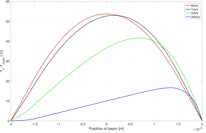
By filling the data from the table 2.1 into equation 2.20, the relation between the velocity of flow and temperature can be described in figure 2.4.

(18)

[image:18.595.106.466.103.334.2]

Figure 2.4: The relation between velocity and temperature. As the flow increases, the temperature profile will shift as same direction as flow.

2.2 Numerical simulations

In this section, the finite element model will be made in COMSOL Multiphysics 5.3 to verify the analytical model. The figure 2.7 shows the overview schematic of the simulation model.

At the inlet and outlet, the temperature is fixed to the room temperature. The heater is replaced in the middle of the channel which can generate the 1 mW

power. To make the Comsol model is comparable with the analytical model, we will use the same parameter as table 2.1.

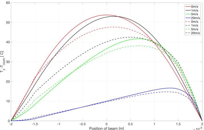
The figure 2.8 shows the COMSOL simulation result. As applying the flow, the temperature profile shift in the same direction as flow. To compare both simula-tions quantitatively, we will subtract the temperature of both simulasimula-tions and then divide by the maximum temperature to calculate the relative average temperature difference, see equation 2.36. For the v = 0m/s, there is 12% relative average

temperature difference between two simulations. For the v = 1m/s, the relative

average temperature difference is 16%. For the v = 5m/s, the relative average

temperature difference different is9.5%and the relative average temperature

differ-ence at v = 20m/s is 8%. The reason behind it is because the geometrical detail

(19)

Figure 2.5: Cross Section of Channel Figure 2.6: Side View of Channel

Figure 2.7: Overview of the simulation schematic.Left: cross section of the tube. Right: side view of the tube

in Matlab will have some difference compare to Comsol simulation.

σtemperature= k=n

P

k=1

(TComsol−Tanalytical)

Tmaximum∗n

(2.36)

[image:19.595.134.491.441.669.2]

In which σtemperature is relative average temperature difference,n is simulation mesh points andTmaximum is maximum temperature of Comsol simulation.

(20)

2.3 Thermal Equation with Different Geometry

To make the analytical model more flexible, in this section, more heaters will be added to the analytical model. Then the analytical model can provide the simulation results for the sensor up to 3 heaters.

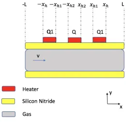
To include the more heaters in the model, we need to recall the heat equation 2.1. The figure2.9 shows the new schematic of thermal flow sensor. Compare to the previous schematic, and there are three heaters placed on the channel, then we can change the value ofQandQ1to determine the number of heaters. At theQ= 0, it

means the sensor includes two heaters, and we even can choose the different heat flux density for these two heaters. At the Q1 = 0, there is only one heater in the

sensor. If we want to simulate the sensor with three heaters, then we can set the Q

[image:20.595.139.400.359.612.2]

andQ1to the value we want.

Figure 2.9: The new geometry of thermal sensor. There are three heater place on the sensor, by changing the Q, we can simulation the model in the

different cases

(21)

T(x) =                                       

A1e

ρcpvx

k +B₁, for−L≤x≤ −x_h (2.37)

C1e

ρcpvx k +C

2 + Q1x ρcpv

, for−xh≤ x≤ −xh1 (2.38) A2e

ρcpvx k +B

2, for−xh1 ≤x≤ −xh2 (2.39) C3e

ρcpvx

k +C₄ +

Qx

ρcpv

, for−xh2 ≤x≤xh2 (2.40) A3e

ρcpvx

k +B₃, forx_h₂ ≤x≤x_h₁ (2.41)

C5e

ρcpvx

k +C₆ +

Q1x ρcpv

, forxh1 ≤x≤xh (2.42)

A4e

ρcpvx

k +B₄, forx_h≤x≤L (2.43)

Where L, xh, xh1, xh2 is indicated in the figure 2.9, Q1 and Q is the heat flux

density of heater.

The similar boundary condition as section 2.1 will be used. Firstly, at x = ±L,

the temperature of the equation is the same as room temperature. Atx=±xh, x= ±xh1, x = ±xh2 , the temperature and heat flux is continuous . Then we can find

(22)

[image:22.595.106.465.102.331.2]

Figure 2.10: The solid line indicate the plot of equation 2.37, and the circle is the plot of equation 2.20. Under the same conditions, the two equations can get the same result.

Compared to the previous mathematical model. The new analytical model should be able to simulate the thermal flow sensor with up to three heaters. In the following section, we will run the analytical simulations for the sensor with a different structure. Again, the Comsol simulations will be used to verify the result.

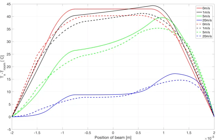
2.3.1 A sensor with two heaters and large gap

Firstly, A sensor with two heaters and a large distance between heaters will be sim-ulated. The simulation will be base on the parameters in table 2.1, in the Table 2.2 only shows the simulation parameter which is different from table 2.1. Figure 2.11 shows the overview schematic of the sensor. The figure 2.12 show the sim-ulation result from Comsol and Matlab. At v = 0m/s,v = 1m/s,v = 5m/s and v = 20m/s, the relative average temperature difference is 7% ,7.5%,7.38% and 7.52%. The main reason cause this difference is the analytical model doesn’t

(23)

[image:23.595.173.425.358.610.2]

Parameters Value Unit Symbol Heater length 1000 um Lheater Gap between two heaters 1000 um Lgap

Table 2.2: The new parameters for two heaters and large gap

(24)

[image:24.595.105.464.262.494.2]

Figure 2.12: The simulation result of the sensor, the dash line indicates the simula-tion result whereas the solid ones indicates the analytical model. Be-cause there is no heater betweenx=−500umandx= 500um,The

temperature remains same at v = 0m/s. As applying the flow, the

(25)

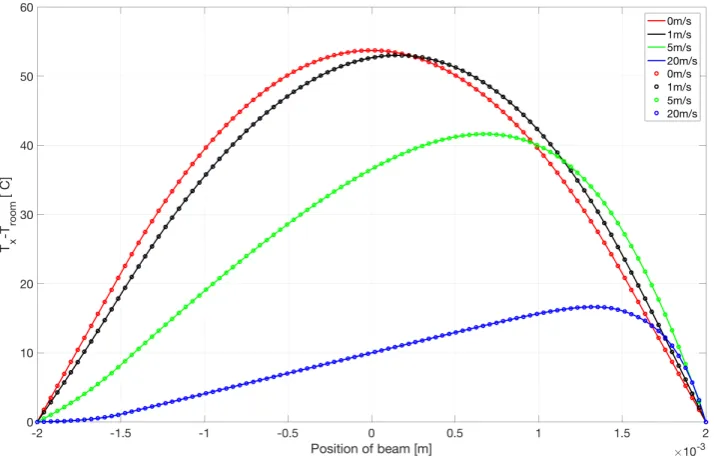
2.3.2 The sensor with one heater in the middle

In this part, the sensor with one heater will be presented. The table 2.3 and figure 2.13 shows the changing parameters of the sensor and an overview schematic of the sensor. The figure 2.14 shows the simulation results, from the figure it can be seen that Comsol simulations gives the almost the same results as the analysis model. Compare to the figure 2.12, the temperature amplitude of one heater design is higher. It can be concluded that as the heater become shorter, the heat flux density will increase.

[image:25.595.168.427.340.589.2]

Parameters Value Unit Symbol Heater length 1000 um Lheater

Table 2.3: The changing simulation parameters for The sensor with one heater

(26)

Figure 2.14: The simulation result of the sensor with one heater in the middle, the dash line indicates the simulation result whereas the solid ones in-dicates the analytical model. At v = 0m/s,v = 1m/s,v = 5m/s

and v = 20m/s, the relative average temperature difference is

(27)

2.3.3 The sensor with more heaters and different heat power

In this section,more complex structures will be presented to see whether the analysis model can predict the temperature profile of the sensor. The table 2.4 and figure 2.15 shows the detail of the sensor. The figure 2.16 shows the simulation results, com-pared to the previous geometry, the simulation results doesn’t fit with the analysis model, and the relative average temperature difference is bigger than the previous two geometries. As the geometry of the sensor becomes more complex, the differ-ence between the calculated effective thermal conductivity and thermal conductivity in Comsol is larger.

Parameters Value Unit Symbol Heater length 500 um Lheater Distance between heaters 500 um Lgap Heat power for the middle heater 1 mW P

Heat power for side heaters 0.5 mW P1

Table 2.4: The new parameters for the sensor with three heaters

Figure 2.15: The sensor with three heaters. The heater in the middle can generated

1mW power, the heat between±xhand±xh1 can generate0.5mW

(28)

Figure 2.16: The simulation result of the sensor with Three heater in the middle, the dash line indicates the simulation result and the solid ones indicates the analytical model.At v = 0m/s,v = 1m/s,v = 5m/s and v = 20m/s, the relative average temperature difference is17%,20%,17%

(29)

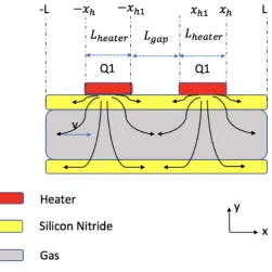
2.4 The Sensor with Heat-sink

If we include the heat-sink, the differential heat equation becomes more compli-cated. Compare to the previous heat equation 2.1, and the new equation will consist of the conductivity of the heat-sink. Thus the equation can be written as:

0 =Acrossk

d2T

dx2 −AcrossρCpv dT

dx −GT +Q

0

(2.44) With Across is area of the channel’s cross section, G is the thermal line con-ductance of the heat-sink in [W/(Km)] and Q0 is line power in [W/(m)]. By

substitutingG0 = _AG cross :

0 =kd 2_T

dx2 −ρCpv dT

dx −G

0

T +Q (2.45)

[image:29.595.163.435.361.672.2]

Now, the temperature profile does not only depend on the flow and beam but also rely on the heat sink, see figure 2.17.

Figure 2.17: The overview schematic of the thermal flow sensor with heat-sink. The blue part indicates the heat-sink which is under the channel.

(30)

T(x) =

                              

A1er1x+B1er2x, for−L≤x≤ −xh (2.46)

C1er1x+C2er2x+ Q1

G0 , for−xh≤x≤ −xh1 (2.47) A2er1x+B2er2x, for−xh1 ≤x≤ −xh2 (2.48) C3er1x+C4er2x+

Q

G0, for−xh2 ≤x≤xh2 (2.49) A3er1x+B3er2x, forxh2 ≤x≤xh1 (2.50) C5er1x+C6er2x+

Q1

G0 , forxh1 ≤x≤xh (2.51) A4er1x+B4er2x, forxh≤x≤L (2.52) Where L,xh,xh1 and xh2 are indicated in the figure 2.9,r1 and r2 are the two

solutions of general solution which can be desirable as:

r1 =

ρcpv

k +

q (ρcpv)2

k2 +

4G0 k

2 (2.53)

r2 =

ρcpv

k −

q (ρcpv)2

k2 +

4G0 k

2 (2.54)

By applying the same boundary condition as previously,14 equations can be found. The solutions can be found in Appendix C.

Next, because the heat-sink is included. Then heat transfer via conduction through the air to the heat sink can be approximated by taking a cylinder [7], see figure 2.18.

G0 = 2∗π∗kair

ln(R_R2₁)∗Across

(2.55)

WithR1andR2is the radius of channel and gap between the channel and heat

sink, kair is the thermal conductivity of air which is 26e−3W/(Km), and Across is the cross section of channel . Then the value of G can be approximated as

2.8e−7_W/₍_Km3₎_.

(31)

[image:31.595.197.484.143.375.2]

Figure 2.18: Method of Images for cylinder approximation

[image:31.595.190.377.564.680.2]

(32)

[image:32.595.90.489.246.485.2]

Figure 2.20: Left: the simulation result of Comsol and Matlab,the dash line indi-cates the simulation result and the solid ones indiindi-cates the analytical model. Atv = 0m/s,v = 1m/s,v = 5m/sandv = 20m/s, the

rel-ative average temperature difference is 5.17%,5.17%,5.45% and 6%.

(33)

[image:33.595.113.514.247.486.2]

Figure 2.21: Left: the simulation result of Comsol and Matlab,the dash line indi-cated the simulation result whereas the solid ones denote the analyt-ical model.At v = 0m/s,v = 1m/s,v = 5m/s and v = 20m/s,

the relative average temperature difference is6%,6%,7.3%and6.5%.

(34)

[image:34.595.87.484.266.480.2]

Figure 2.22: Left: the simulation result of Comsol and Matlab,the dash line indi-cated the simulation result whereas the solid ones denote the analyt-ical model.At v = 0m/s,v = 1m/s,v = 5m/sand v = 20m/s, the

relative average temperature difference is5.6%,5.6%,6.2%and4.7%.

(35)

(36)

2.5 Overview

(37)

Bronkhorst Sensors

This chapter describes the design, simulation, fabrication, and characterization of the thermal flow sensor developed in collaboration with the Bronkhorst. The sec-tion ends with a discussion of the results and suggessec-tions for the new thermal flow sensor.

3.1 Design

There are three types of the sensor designed by Bronkhorst, and all of them have two heaters on the channel, which can heat the channel up and measure the tem-perature changes. The next section will describe the important structures of each sensor.

3.1.1 The design with different diameters of channel

Firstly, the thermal flow sensor with different channel diameters will be introduced, see figure 3.1. The important structures are denoted as:

1. The channel with 31umradius.

4. Inlet.

5. Outlet.

6. Pressure sensor.

7. Pressure sensor.

(38)

38 CHAPTER3. BRONKHORSTSENSORS

Figure 3.1: The sensor with different channel diameters, the dash block 1 is the channel with 31.5um, the dash block 2 is the channel with 45umand

the last one is the channel with 55um.

To fabricate the channel with different radii, different densities of patterns (purple) will be used on the device layer, see figure 3.2.The design parameters can be found in table 3.1.

Parameters Value Unit

Heater’s dimension(Hheater∗Wheater∗Lheater) 0.2×95×1500 um

Resistance of heater 500 Ω

Tube length 4000 um

Radius of channel 1 31.5 um

Radius of channel 2 45 um

[image:38.595.90.330.83.319.2]

Radius of channel 3 55 um

(39)

Figure 3.2: The overview of the schematics of the channels. The channel with 31.5

umradius have one line patterns on the device layer, the channel with

45umradius have two lines patterns on the device layer and the

chan-nel with 55umradius have three lines patterns on the device layer.

3.1.2 The Sensor with Different Heater Length

In this section, the sensor with different heater’s length will be presented. Under the same supply voltage, the short heater will generate more power than the long heater. The sensor is designed as figure 3.3. The important structures are denoted as:

1. The heater with 500um.

2. The heater with 1000umradius.

3. The heater with 1500umradius.

4. Inlet.

5. Outlet.

6. Pressure sensor.

7. Pressure sensor.

(40)

Figure 3.3: The sensor with different heater length. The dash block 1 is the channel with 500 um heater, the dash block 2 is the channel with 1000 um

heater and the dash block 3 is the channel with 1500um.

Heater1’s dimension(Hheater∗Wheater∗Lheater) 0.2×95×500 um Resistance of 500umheater 200 Ω

[image:40.595.89.334.127.361.2]

Radius of channel 31.5 um

(41)

3.1.3 The design with parallel channels

The third sensor is designed with several parallel channels, the purpose of this de-sign is to reduce the pressure drop of fluid and increase the measurement range. For each channel, there is the 1500um heater replace on the channel. The sensor

layout is shown in figure 3.4, and the important structures are denoted as:

1. 3 Parallel Channels . 2. 5 Parallel Channels . 3. Pressure Sensor. 4. Pressure Sensor. 5. Inlet.

[image:41.595.196.410.373.584.2]

6. Outlet.

Figure 3.4: The sensor with parallel channels.

(42)

Heater’s dimension(Hheater∗Wheater∗Lheater) 0.2×95×500 um Resistance of 3 parallel channel 1500 Ω

Resistance of 5 parallel channel 2500 Ω

Tube length 4000 um

Radius of channel 31.5 um

Table 3.3: The design parameter for thermal flow sensor with parallel channels

3.2 Fabrication Process

Figures 3.5 , 3.6 and 3.7 show the fabrication process of the sensor. The process starts with depositing SiRN layer by using low-pressure chemical vapor deposition. Then the chromium is sputtered to protect the SiRN during the channel etch. Next, a photoresist layer is deposited and patterned; the pattern will determine the shape and size of the channel. The channel will be etched by using a semi-isotropicSF6.

Then the resist and chromium will be removed. Instead, a layer of silicon dioxide is deposited by using LPCVD, and the silicon dioxide layer will prevent etching the channel during the inlet and outlet etch.

The inlet and outlet are etched by using reactive-ion etching(DRIE), and the sil-icon dioxide layer will protect the channel from etching. Next, the silsil-icon dioxide is removed using wet etch, and the SiRN layer is deposited to cover the channel and access, using LPCVD. Afterwards, a 200 nm thick metal layer is sputtered at the

topside of the channel. Last, the channel is released from the bulk.

(43)

[image:43.595.206.422.132.670.2]

(44)

[image:44.595.179.390.225.582.2]

(45)

3.3 Specific readout design

In the real design, there are four heaters assembled on one ”U” shaped tube as is shown in figure 3.8, and all heaters will heat up to the same temperature when there is no flow applied. As applying the flow, the distribution of temperature will be shifted in the flow direction. This temperature shift will change the heater’s resistance which can be described as following equation [8] [9]:

Figure 3.8: The configuration of the channel, in the figure the red part is the heater and measurement resistor, and these four heaters will be connected as Wheatone Bridge

R(T) =R0[1 +α∆T] (3.1)

∆T = ∆R

αR0

(3.2) Where the R0 is the heater’s resistance at T = Troom, ∆T the temperature

difference betweenT andTroom, andαthe temperature coefficient of resistance of

the heater.

To measure the resistance changes in the equation 3.2, the Wheatstone-bridge will be used. Figure 3.9 shows the configuration of the circuit and the mathematical equations of this circuit can be described as following:

Voutput = (

Rdown

Rdown+Rup

− Rup

Rdown+Rup

(46)

To simplify the equation 3.3, theRdown andRup can be described as:

Rup =R0+ ∆TupαR0 (3.4)

Rdown =R0+ ∆TdownαR0 (3.5)

Where∆Tdownand∆Tupis the average temperature difference on the upstream and downstream. Then the equation 3.3 can be described :

Voutput =Vbridge∗

(∆Tdown−∆Tup)α

2 + (∆Tdown + ∆Tup)α

[image:46.595.100.471.284.530.2]

(3.6)

(47)

3.4 Measurement Result

In this section, the measurement result will be presented and compared to the sim-ulation result. The silicon nitride layer and the gold layer are regarded as thin film material. Then in the later on in simulation, the thermal conductivity of silicon ni-tride will be 3 W/Km [10]. The TCR of gold is 0.00147/K which comes from

measuring.

Furthermore, the sensor with parallel channels is not working during the mea-surement, in this section, only the results coming from the working sensor will be presented and discussed. To compare the different simulation results, all the simu-lations will use the same volumetric flow rate as the measurement. Again, we will subtract the simulation result from the measurement result, and divided by the max-imum voltage output of Comsol to calculate the relative average voltage difference.

Some parameters will be changed to get an understanding of how they influence the sensitivity and measurement range of the sensor. Figure 3.10 shows how to define the sensitivity and measurement range of the sensor. The measurement range is the range of this linear part, and the slope of this linear line can be defined as sensitivity.

(48)

3.4.1 Simulation and Measurement Result of Sensor with

Differ-ent Diameter Channel

In this section, the sensor with different diameters will be tested and simulated, to make sure the simulation is in the same conditions as the real measurement, the simulation parameters as table 3.4 will be used. Furthermore, to ensure the Matlab simulation have the proper heat-sink structure, the thermal conductance of heat-sink will directly be derived from Comsol simulation.

Thermal Conductivity of Silicon Nitride 3 W/Km

TCR of Gold 0.00147 1/K

Thermal Conductivity of Gold Thin Flim [11] 80 W/Km

Bridge Voltage of Wheatone Bridge 956 mV

Heater’s Length 1500 um

Ambient Temperature 293.15 K

Amplification Factor 150

Table 3.4: The Simulation Parameters

The Sensor with 31.5 um Radius Channel

The results of measurement and simulation are shown in figure 3.11.

TheG0 = 14e6W/Km3 is derived from Comsol simulation, the Comsol simulation

and Matlab simulation is close to each other, but there is an unexpected drop in flow velocity 28m/s and 29m/s. To investigate the reason, we increased sweep steps

and mesh density, but this unexpected drop is still in the figure, thus it might be for some specific value the Comsol can’t give a proper result.

But for both simulation results, there is around20% different from the

measure-ment result, because the channel is placed on the position where there is a silicon wall on one side and another side is air, thus the heat-sink structure of measurement sensor is more complicated than the simulation structure. It is too difficult to build the same heat-sink structure as the actual sensor in the Comsol and Matlab.

(49)

Figure 3.11: The results of different sensor for 31.5um radius channel. The blue

line indicates the simulation result from analytical model, the red line indicates the Comsol simulation, the pink one indicates the ment result from chip 4.6 and the black line indicates the measure-ment result from chip 9.8. The relative average voltage difference with respect to measurement data and analysis data of chip 4.6 is 21%,

(50)

the measurement result and Matlab result with adjusted conductance coefficient with

G0 = 19e6W/Km3.

Figure 3.12: The result of analytical model and measurement, the blue line indi-cates the result of analytical Model and the pink point is the mea-surement result. In this simulation G0 = 19e6W/Km3_{.The relative}

(51)

The Sensor with 45 um Radius Channel

The results of the channel with 45um radius channel is shown in figure 3.13, The G0 = 8.7e6W/Km3 _{. From the figure, it can be seen that the difference between}

measurement value and simulation is smaller than the sensor with 45um radius

channel. Since theG0 =G/Across, as the radius of the channel increases, the

ther-mal conductivity line increases, and meanwhile the cross-section area increases, but when the change rate of the cross section is bigger than the change rate of thermal conductivity, then the cross-section area will dominate the equation. This changes will result in theG0 decrease. Thus there is less influence from the

heat-sink structure.

Figure 3.13: The results of simulation and measurement for45umradius channel.

The blue line indicates the simulation result from analytical model, the red line indicates the Comsol simulation and the black one indicate the measurement result. The relative average voltage difference with re-spect to measurement data and analysis data is12%, and the relative

average voltage difference with respect to Comsol data and measure-ment data is 11%.The sensitivity of the sensor is 48mV /(ml/min)

(52)

The Sensor with 55 um Radius Channel

This section describes how the sensitivity of the sensor is influenced by changing the heater’s length. As with the previous measurement with the variation of the channel’s radius, the simulation parameters should be the same for Matlab and Comsol. The table 3.5 shows the simulation parameters. Furthermore, the G0 will also directly

derived from Comsol simulation.

Figure 3.14: The results of simulation and measurement for 55um radius

chan-nel. The blue line indicates the simulation result from analytical model, the red line indicates the Comsol simulation and the black one in-dicate the measurement result. The relative average voltage differ-ence with respect to measurement data and analysis data is 6.18%,

(53)

3.4.2 Simulation and Measurement Result of Sensor with

Differ-ent Heater Length

In this section, we will change the heater’s length to investigate how it will influence the sensitivity of the sensor. As with the previous measurement with the variation of the channel’s radius, the simulation parameters should be the same for Matlab and Comsol. But in this section, as the length of heater decreases, the resistance of heaters will decreases as well, and the heater can generate more power. The table 3.5 shows the simulation parameter. Furthermore, the heat-sink conductance will also directly derived from Comsol simulation.

Radius of Channel 31.5 um

Power of1500umheater 0.418 mW

(54)

The Sensor with 1500 um heater length

Firstly, the sensor with 1500 um heater will be measured. The figure 3.15 shows

the simulation result and measurement result. Because of the difference of heat-structure between the simulation model and sensor, there still is some difference between the simulation result and measuring result. The figure 3.16 shows the simulation result of the adjusted heat-sink value, the G0 = 18e6W/Km3_{, and the}

relative average voltage difference is1.5%.

Figure 3.15: The result of simulation and measurement for the sensor with1500um

heater.The blue line indicates the simulation result from analytical model, the red line indicates the Comsol simulation and the black one indicate the measurement result. The relative average voltage differ-ence with respect to measurement data and analysis data is 12.68%,

(55)

Figure 3.16: The result of Matlab Model and measurement, the blue line indicates the result of Matlab Model and the pink line is the measurement result. In this simulation the conduction of heat sink is18e6W/Km3, and the

relative average voltage difference is1.5%

Secondly, the sensor with 1000umheater length is simulated and measured. The

figure 3.17 shows the simulation and measuring result. Compared to the sensor with 1500 umheater length, the sensitivity of the sensor is improved, because the

heat flux density is increasing as the length of heater decreasing. But there still some difference between the simulation result and measurement result, because of the difference of the heat-sink structure. But compared to the sensor with 1500um

(56)

heater.The blue line indicates the simulation result from analytical model, the red line indicates the Comsol simulation and the black one indicate the measurement result. In this simulation the G0 = 15.4e6W/Km3.The relative average voltage difference with respect

to measurement data and analysis data is6.2%, and the relative

aver-age voltaver-age difference with respect to Comsol data and measurement data is 5.2%.The sensitivity of the sensor is 118mV /(ml/min)and

(57)

The last sensor is fabricated with 500 um heater length, the simulation and

mea-surement result can be found in figure 3.18. TheG0 = 15.4e6W/Km3_{. When the}

heater becomes shorter, the temperature difference between the upstream heater and downstream heater is increasing in length. Meanwhile, the sensitivity is also increasing. The relative average voltage difference between the simulation result and the measurement result is7%(Analytical model) and5.14%(Matlab model).

heater.The blue line indicates the simulation result from analytical model, the red line indicates the Comsol simulation and the black one indicate the measurement result. The relative average voltage dif-ference with respect to measurement data and analysis data is 7%,

(58)

3.5 The Prediction of Parameter’s Influence

An excellent thermal flow sensor should have high sensitivity, large measurement range, and low-pressure drop. In the last sections, we have already investigated the how the behavior of sensor changes with changing radius and heater’s length. However, there are still a lot of parameters that can influence the performance of the sensor. For example, the position of the heater can be adjusted, the channel length can be adjusted, etc. In this section, we will change some parameters to see how it influence the behavior of the sensor.

3.5.1 Distance Between Heaters

Firstly, the distance between the two heaters will be adjusted to investigate how it influences the performance of the sensor. The simulation parameters will be the same as the sensor with 1500um, 1000um and 500um the heater length which

presented in the last section, and the distance between two heaters will be changed from0umto200um. The table 3.6 shows the simulation parameters.

Table 3.6: The simulation parameters for the model with changing distance between two heaters.

From the figure 3.19, as the distance between heaters increases, the sensitivity of the sensor will decreases. The reason behind it is as the distance between the heaters increase, the temperature drop between the two heaters will also increase, the temperature profile shows in appendix D.

(59)

[image:59.595.137.494.94.317.2]

Figure 3.19: The simulation result with changing the distance between the two heaters. The first figure is the heater with 500 um length, and the

distance is changed from 0umto 200 um. The second figure is the

sensor with 1000umheater and the third one is the sensor with 1500 umheater.

3.5.2 Channel length

In the analytical model, the length of the channel is one of the variables in the heat equation. Thus it is interesting to know how the length of the channel influences the sensitivity. Firstly the simulation parameters will be defined, the heater’s length will be chosen as500um and without any gap between two heaters, and the length of

the channel will changes from 4000 to 1000um. And the rest of the parameters will

be the same as 3.6.

Figure 3.20 shows the simulation result. For the 4000um, 3000umand 2000 um, the output voltage remains at same level. But from the 1800 um, the output

(60)

Figure 3.20: The simulation results of changing channel length. The triangle mark is the sensor with 4000umchannel length, the blue cross is the sensor

with 3000 um channel length, the blue solid line is the sensor with

2000umchannel length and red line is s the sensor with 1000um

3.5.3 How the fabrication process influence the performance

During the fabrication process, it is difficult to make sure the thickness of the material is the same as it supposes to be. Since some material such as the heater and the SiRN wall are regarded as thin film material,the changing the thickness will cause the properties of the material to change. Thus, in this section, we will investigate how the material properties influences the performance of the sensor. The simulation parameters can be found in table 3.7.

G0 20 W/(km3)

Length of heater 500 um

Length of Channel 2000 um

(61)

Figure 3.21: The simulation result of changing effective thermal conductivity.

Firstly, the thermal conductivity of SiRN will increase from3W/mKto9W/mK.

The figure 3.21 shows the simulation result, as the thermal conductivity of SiRN increases the sensitivity of the sensor decrease.

(62)

Figure 3.22: The simulation result of changing TCR of gold.

3.6 Overview

This chapter presents both simulation results and the measurement results. There still some differences between the simulation results and measurement results. The reason behind it is we can’t build the same heat-sink structure as the real sensor, and calculation value of theG0 will be different from the actual sensor. However, we

can adjust theG0 to fit the measurement result, which also means if we can get the

accurate value for the conductivity of heat-sink, the simulation model can predict the output of sensor accurately.

(63)

Conclusion and Discussion

This thesis presents two types of model to predict the behavior of a thermal flow sensor. The first model is built in Comsol, which is using numerically way to calculate the temperature profile of the sensor. The advantages of Comsol is that it can create the model in 3D, and it can use the multiple physical models. But it takes a long time to finish the simulation, especially if there is any thin film structure in the model, we must increase the mesh size to get an accurate result, and it will result in even longer time consumption. The second model is an analytical model which based on the heat equation. The advantage of the analytical model is that it takes much less time to generate the result, and the result is close to the Comsol simulation.

Later on, the sensors from the Bronkhorst are measured to verify the simulation results. The simulation result is close to the measurement result, but there is some difference between the simulation result and measurement result. The main reason behind it is that the heat structure in the actual sensor is too complex to construct it in the simulation. Meanwhile, we also investigate how the design parameters will influence the behavior of the thermal flow sensor. From the simulation and mea-surement result in chapter 3.4.1, the sensitivity of the sensor increases as the radius increases. For example, the sensitivity of the sensor with31.5umradius channel is

40.6mV /(ml/min), when we increase the radius of channel to 45um, the

sensi-tivity now is 48mV /(ml/min). In the chapter 3.4.2, the sensitivity of the sensor

can be improved by decreasing the heater’s length. For example, the sensitivity of the sensor with1000umheater is118mV /(ml/min), the sensitivity of the sensor

with500umheater is250mV /(ml/min). Except for these two parameters, there

still have some parameters can influence the behavior of the sensor. Thus, in chap-ter 3.5, we run the analytical model by adjusting some design paramechap-ters, such as the distance between two heaters, channel length, and material properties. It turns out that increasing the distance of two heaters, decreases the channel length and increases the thickness of SiRN will result in decreasing the sensitivity. By collecting all these information, the new thermal sensor with one heater is designed. But due

(64)

64 CHAPTER4. CONCLUSION AND DISCUSSION

(65)

Outlook on future work

In this thesis, the analytical model is built to predict the behavior of the thermal flow sensor, but there are some items remain to be done:

1. The equation to approximate the G0 in this thesis is not accurate enough,

therefore it is important to find a proper way to calculate theG0.

2. Except the design parameters mentioned in this thesis, there still have some design parameters can be investigated, for example, it might help to place the sensor in the vacuum, the sensitivity might be improved by applying more heaters, the measurement range might be an increase by using multiple chan-nels, etc.

3. Base on the analytical model in this thesis, it might be interesting to develop a software can generate omptimal design parameter when we enter the sensi-tivity and measurement range.

(66)

(67)

[1] “Comsol, inc.” https://www.comsol.com/. [2] “Ansys, inc.” https://www.ansys.com/.

[3] J. Groenesteijn, M. J. de Boer, J. C. L¨otters, and R. J. Wiegerink, “A versatile technology platform for microfluidic handling systems, part i: fabrication and functionalization,” Microfluidics and Nanofluidics, vol. 21, no. 7, p. 127, Jul

2017. [Online]. Available: https://doi.org/10.1007/s10404-017-1961-0 [4] “Bronkhorst nederland b.v.” https://www.bronkhorst.nl/.

[5] H.H.Bruun.,Hot-Wire Anemometry. Oxford University Press, 1994.

[6] “Wolfram research corp.” http://www.wolfram.com/.

[7] T. L. B. A. S. L. Frank P. Incropera, David P. Dewitt,Fundamentals of Heat and Mass Transfer. JOHN WILEY SONS, 2006.

[8] K. Ohe and Y. Naito, “A new resistor having an anomalously large positive tem-perature coefficient,”Japanese Journal of Applied Physics, vol. 10, no. 1, p. 99,

1971.

[9] A. Alenitesyn and E. Butikov, “. concise handbook of mathematics and physics.”

CRC Press (Boca Raton, Fla. and Moscow), 1997.

[10] C. H. Mastrangelo, Y.-C. Tai, and R. S. Muller, “Thermophysical properties of low-residual stress, silicon-rich, lpcvd silicon nitride films,” Sensors and Actuators A: Physical, vol. 23, no. 1, pp. 856 – 860, 1990, proceedings

of the 5th International Conference on Solid-State Sensors and Actuators and Eurosensors III. [Online]. Available: http://www.sciencedirect.com/science/ article/pii/092442479087046L

[11] G. Langer, J. Hartmann, and M. Reichling, “Thermal conductivity of thin metallic films measured by photothermal profile analysis,” Review of Scientific Instruments, vol. 68, no. 3, pp. 1510–1513, 1997. [Online]. Available:

https://doi.org/10.1063/1.1147638

(68)

(69)

The method to solve the constants

In this section, we will present the way to solve the equation 2.23 to 2.28 in section 2.1:

A1e−rL+B1 =A2erL+B2 =Theatsink (A.1)

A1e−rxh +B1 =C1e−rxh +C2− Qxh

rk (A.2)

A2erxh +B2 =C1erxh +C2+ Qxh

rk (A.3)

A1re−rxh =C1re−rxh + Q

rk (A.4)

A2rerxh =C1rerxh+ Q

rk (A.5)

To solve the six constant,firstly we rewrite the equation A.1 as following:

A1e−rL−A2erL =B2−B1 (A.6)

Then using equation A.3 minus A.2:

A2erxh −A1e−rxh +A1e−rL−A2erL =C1erxh −C1e−rxh + 2 Qxh

rk (A.7)

Next using equation A.5 minus A.4 to find the relation betweenC1 ,A1 andA2

A2rerxh −A1re−rxh =C1erxh −C1e−rxh (A.8)

Replacing the equation A.8 into A.7, the relation between A1 and A2 can be

found as:

A1 = 2 Qxh

rke−rL +A2e

2rL _(A.9)

(70)

70 APPENDIX A. THE METHOD TO SOLVE THE CONSTANTS

To solve theA1 and A2 we need using euqaiton A.4 and A.5 again, but before

subtracting them, the equation A.4 need to divide e−rxh and the equation A.5 need

to divideerxh:

A1−A2 =

Q

r2_ke−rxh

− Q

r2_kerxh (A.10)

Replacing equation A.9 into A.10 theA2 can be solved as:

A2 =

Q(e−r(L−xh)₋_e−r(L+xh)₋₂_x

hr)

r2_k₍_erL₋_e−rL₎ (A.11) Now we have already knownA2, then theA1can be solved by replacingA2into

equation A.10,C1 can be solved by replacingA1 andA2 into equation A.8, and B1

(71)

The constant for equation 2.37

This section provide the constants for the heat equation 2.37, which is located in Chapter 2.3.

It is difficult to solve the 14 variables with 14 equations, then the software called Mathematica is used to solve the equation, the PDF file attached as following shows those 14 equations and the solution of them.

(72)

解方程

SolveA1×ⅇ-r*L+B1⩵0 && A4×ⅇr*L+B4 ⩵0 &&

A1×ⅇ-r*Xh+B1-C1×ⅇ-r*Xh-C2+Q×Xh  r×k ⩵0 &&

A1×r×ⅇ-r*Xh-C1×r×ⅇ-r*Xh-Q  r×k ⩵0 &&

A2×ⅇ-r*Xh1+B2-C1×ⅇ-r*Xh1-C2+Q×Xh1  r×k ⩵0 &&

A2×r×ⅇ-r*Xh1-C1×r×ⅇ-r*Xh1-Q  r×k ⩵0 &&

A2×ⅇ-r*Xh2+B2-C3×ⅇ-r*Xh2-C4+Q×Xh2  r×k ⩵0 &&

A2×r×ⅇ-r*Xh2-C3×r×ⅇ-r*Xh2-Q  r×k ⩵0 &&

A3×ⅇr*Xh2+B3-C3×ⅇr*Xh2-C4-Q×Xh2  r×k ⩵0 &&

A3×r×ⅇr*Xh2-C3×r×ⅇr*Xh2-Q  r×k ⩵0 &&

A3×ⅇr*Xh1+B3-C5×ⅇr*Xh1-C6-Q×Xh1  r×k ⩵0 &&

A3×r×ⅇr*Xh1-C5×r×ⅇr*Xh1-Q  r×k ⩵0 &&

A4×ⅇr*Xh+B4-C5×ⅇr*Xh-C6-Q×Xh  r×k ⩵0 &&

A4×r×ⅇr*Xh-C5×r×ⅇr*Xh-Q  r×k ⩵0,

{A1, B1, A2, B2, A3, B3, A4, B4, C1, C2, C3, C4, C5, C6}

A1 →

1

-1+ⅇ2 L rk r2 ⅇ

L r-r Xh-r Xh1-r Xh2_Q

-ⅇL r+r Xh+r Xh1₊_ⅇL r+r Xh+r Xh2_-_ⅇL r+r Xh1+r Xh2₊_ⅇL r+2 r Xh+r Xh1+r Xh2_-_ⅇL r+r Xh+2 r Xh1+r Xh2₊

ⅇL r+r Xh+r Xh1+2 r Xh2_-₂_ⅇr Xh+r Xh1+r Xh2_{r X}

h+2ⅇr Xh+r Xh1+r Xh2r Xh1-2ⅇr Xh+r Xh1+r Xh2r Xh2,

B1 →

-1

-1+ⅇ2 L rk r2 ⅇ

-r Xh-r Xh1-r Xh2_Q_-_ⅇL r+r Xh+r Xh1₊_ⅇL r+r Xh+r Xh2_-_ⅇL r+r Xh1+r Xh2₊

ⅇL r+2 r Xh+r Xh1+r Xh2_-_ⅇL r+r Xh+2 r Xh1+r Xh2₊_ⅇL r+r Xh+r Xh1+2 r Xh2

-2ⅇr Xh+r Xh1+r Xh2_{r X}

h+2ⅇr Xh+r Xh1+r Xh2r Xh1-2ⅇr Xh+r Xh1+r Xh2r Xh2,

A2 →

1

-1+ⅇ2 L rk r2 ⅇ

-r Xh-r Xh1-r Xh2_Q_-ⅇ2 L r+r Xh+r Xh1₊_ⅇ2 L r+r Xh+r Xh2_-_ⅇ2 L r+r Xh1+r Xh2₊

ⅇ2 r Xh+r Xh1+r Xh2_-_ⅇr Xh+2 r Xh1+r Xh2₊_ⅇ2 L r+r Xh+r Xh1+2 r Xh2

-2ⅇL r+r Xh+r Xh1+r Xh2_{r X}

h+2ⅇL r+r Xh+r Xh1+r Xh2r Xh1-2ⅇL r+r Xh+r Xh1+r Xh2r Xh2,

B2 →

1

-1+ⅇ2 L rk r2 ⅇ

-r Xh-r Xh1-r Xh2_Q_ⅇL r+r Xh+r Xh1_-_ⅇL r+r Xh+r Xh2₊_ⅇL r+r Xh1+r Xh2

-ⅇL r+2 r Xh+r Xh1+r Xh2₊_ⅇL r+r Xh+2 r Xh1+r Xh2_-_ⅇL r+r Xh+r Xh1+2 r Xh2₊_ⅇr Xh+r Xh1+r Xh2_{r X} h+

ⅇ2 L r+r Xh+r Xh1+r Xh2_{r X}

h-ⅇr Xh+r Xh1+r Xh2r Xh1-ⅇ2 L r+r Xh+r Xh1+r Xh2r Xh1+2ⅇr Xh+r Xh1+r Xh2r Xh2,

A3 →

1

-1+ⅇ2 L rk r2 ⅇ

-r Xh-r Xh1-r Xh2_Q_-ⅇr Xh+r Xh1₊_ⅇ2 L r+r Xh+r Xh2_-_ⅇ2 L r+r Xh1+r Xh2₊

ⅇ2 r Xh+r Xh1+r Xh2_-_ⅇr Xh+2 r Xh1+r Xh2₊_ⅇr Xh+r Xh1+2 r Xh2_-₂_ⅇL r+r Xh+r Xh1+r Xh2_{r X} h+

2ⅇL r+r Xh+r Xh1+r Xh2_{r X}

h1-2ⅇL r+r Xh+r Xh1+r Xh2r Xh2,

B3 →

1

-1+ⅇ2 L rk r2 ⅇ

-r Xh-r Xh1-r Xh2_Q_ⅇL r+r Xh+r Xh1_-_ⅇL r+r Xh+r Xh2₊_ⅇL r+r Xh1+r Xh2_-_ⅇL r+2 r Xh+r Xh1+r Xh2₊

ⅇL r+r Xh+2 r Xh1+r Xh2_-_ⅇL r+r Xh+r Xh1+2 r Xh2₊_ⅇr Xh+r Xh1+r Xh2_{r X}

h+ⅇ2 L r+r Xh+r Xh1+r Xh2r Xh

-ⅇr Xh+r Xh1+r Xh2_{r X}

h1-ⅇ2 L r+r Xh+r Xh1+r Xh2r Xh1+2ⅇ2 L r+r Xh+r Xh1+r Xh2r Xh2,

(73)

A4 →

1

-1+ⅇ2 L rk r2 ⅇ

-r Xh-r Xh1-r Xh2_Q_-ⅇr Xh+r Xh1₊_ⅇr Xh+r Xh2_-_ⅇr Xh1+r Xh2₊

h1-2ⅇL r+r Xh+r Xh1+r Xh2r Xh2, B4→

-1

-1+ⅇ2 L rk r2

ⅇL r-r Xh-r Xh1-r Xh2_Q_-_ⅇr Xh+r Xh1₊_ⅇr Xh+r Xh2_-_ⅇr Xh1+r Xh2₊_ⅇ2 r Xh+r Xh1+r Xh2_-_ⅇr Xh+2 r Xh1+r Xh2₊

ⅇr Xh+r Xh1+2 r Xh2_-₂_ⅇL r+r Xh+r Xh1+r Xh2_{r X}

h+2ⅇL r+r Xh+r Xh1+r Xh2r Xh1-2ⅇL r+r Xh+r Xh1+r Xh2r Xh2,

C1 →

-1

-1+ⅇ2 L rk r2 ⅇ

-r Xh-r Xh1-r Xh2_Q_ⅇ2 L r+r Xh+r Xh1_-_ⅇ2 L r+r Xh+r Xh2₊_ⅇ2 L r+r Xh1+r Xh2

-ⅇ2 r Xh+r Xh1+r Xh2₊_ⅇ2 L r+r Xh+2 r Xh1+r Xh2_-_ⅇ2 L r+r Xh+r Xh1+2 r Xh2₊

h-2ⅇL r+r Xh+r Xh1+r Xh2r Xh1+2ⅇL r+r Xh+r Xh1+r Xh2r Xh2,

C2 →

1

-1+ⅇ2 L rk r2 ⅇ

-ⅇr Xh+r Xh1+r Xh2₊_ⅇ2 L r+r Xh+r Xh1+r Xh2_-_ⅇL r+2 r Xh+r Xh1+r Xh2₊_ⅇL r+r Xh+2 r Xh1+r Xh2_-_ⅇL r+r Xh+r Xh1+2 r Xh2₊

ⅇr Xh+r Xh1+r Xh2_{r X}

h+ⅇ2 L r+r Xh+r Xh1+r Xh2r Xh-2ⅇr Xh+r Xh1+r Xh2r Xh1+2ⅇr Xh+r Xh1+r Xh2r Xh2,

C3 →

1

-1+ⅇ2 L rk r2 ⅇ

-r Xh-r Xh1-r Xh2_Q_-ⅇ2 L r+r Xh+r Xh1₊_ⅇ2 L r+r Xh+r Xh2_-_ⅇ2 L r+r Xh1+r Xh2₊

h1-2ⅇL r+r Xh+r Xh1+r Xh2r Xh2,

C4 →

1

-1+ⅇ2 L rk r2 ⅇ

-ⅇr Xh+r Xh1+r Xh2₊_ⅇ2 L r+r Xh+r Xh1+r Xh2_-_ⅇL r+2 r Xh+r Xh1+r Xh2₊_ⅇL r+r Xh+2 r Xh1+r Xh2_-_ⅇL r+r Xh+r Xh1+2 r Xh2₊

h+ⅇ2 L r+r Xh+r Xh1+r Xh2r Xh-ⅇr Xh+r Xh1+r Xh2r Xh1-ⅇ2 L r+r Xh+r Xh1+r Xh2r Xh1+

h2+ⅇ2 L r+r Xh+r Xh1+r Xh2r Xh2, C5 →

-1

-1+ⅇ2 L rk r2

ⅇ-r Xh-r Xh1-r Xh2_Q_ⅇr Xh+r Xh1_-_ⅇr Xh+r Xh2₊_ⅇ2 L r+r Xh1+r Xh2_-_ⅇ2 r Xh+r Xh1+r Xh2₊_ⅇr Xh+2 r Xh1+r Xh2

-ⅇr Xh+r Xh1+2 r Xh2₊₂_ⅇL r+r Xh+r Xh1+r Xh2_{r X}

h-2ⅇL r+r Xh+r Xh1+r Xh2r Xh1+2ⅇL r+r Xh+r Xh1+r Xh2r Xh2,

C6 →

1

-1+ⅇ2 L rk r2 ⅇ

-r Xh-r Xh1-r Xh2_Q_ⅇL r+r Xh+r Xh1_-_ⅇL r+r Xh+r Xh2₊_ⅇL r+r Xh1+r Xh2_-_ⅇr Xh+r Xh1+r Xh2₊

ⅇ2 L r+r Xh+r Xh1+r Xh2_-_ⅇL r+2 r Xh+r Xh1+r Xh2₊_ⅇL r+r Xh+2 r Xh1+r Xh2_-_ⅇL r+r Xh+r Xh1+2 r Xh2₊_ⅇr Xh+r Xh1+r Xh2

r Xh+ⅇ2 L r+r Xh+r Xh1+r Xh2r Xh-2ⅇ2 L r+r Xh+r Xh1+r Xh2r Xh1+2ⅇ2 L r+r Xh+r Xh1+r Xh2r Xh2

(74)

(75)

The constant for equation 2.46

The solution for the equation 2.46,as describe in the chapter 2.4. The constant is solved by using Mathmematica ,reads: