University of Warwick institutional repository: http://go.warwick.ac.uk/wrap
A Thesis Submitted for the Degree of PhD at the University of Warwick
http://go.warwick.ac.uk/wrap/3714
This thesis is made available online and is protected by original copyright. Please scroll down to view the document itself.
M A
E
G NS
I T A T MOLEM
U N
IV ER
SITAS WARWICEN
SIS
Modelling Techniques for the study of
Molecular Self-Organisation
by
Sara Fortuna
Thesis
Submitted to the University of Warwick
for the degree of
Doctor of Philosophy
What could we do with layered structures with just the right layers?
What would the properties of materials be if we could really arrange the atoms the way
we want them? They would be very interesting to investigate theoretically. I can’t see
exactly what would happen, but I can hardly doubt that when we have some control of
the arrangement of things on a small scale we will get an enormously greater range of
possible properties that substances can have, and of different things that we can do.
(Richard P. Feynman - annual meeting of the American Physical Society
at the California Institute of Technology - December 29th 1959)
Table of Contents
List of Figures . . . iv
List of Tables . . . vi
Acknowledgments . . . vii
Declaration and Inclusion of Material from a Prior Thesis . . . viii
Abstract 1 Abbreviations . . . 2
1 Introduction 3 1.1 Self-Organisation in Chemistry . . . 3
1.2 Molecular Systems as Multiscale Complex Systems . . . 6
1.3 Aim of this Work . . . 7
1.4 Thesis Outline . . . 8
2 Modelling Techniques and Theoretical Background 9 2.1 Model Systems . . . 9
2.1.1 Lattice Models . . . 9
2.1.2 Rigid-Soft Models . . . 12
2.1.3 Molecular Mechanics Based Models . . . 14
2.2 Some Statistical Mechanics Definitions . . . 16
2.3 Simulation Methods in Chemistry . . . 17
2.3.1 Deterministic Methods: Molecular Dynamics . . . 17
2.3.2 Stochastic Methods: Monte Carlo . . . 19
2.3.3 Multiscale Methods . . . 22
2.4 Simulation Methods in Complexity Science . . . 23
2.4.1 Genetic Algorithms . . . 24
2.4.2 Cellular Automata . . . 25
2.4.3 Rule Based Artificial Intelligence: Agents . . . 26
3 Monte Carlo Simulation of Polydisperse Spheres on a Spherical Surface 28 3.1 The Sphere Packing Problem . . . 28
3.2 Synthesis of Coated Nanoparticles . . . 29
3.4 Conclusion . . . 37
4 2D Hexagonal Lattice Model for the Hydrogen-Bonded Driven Self-Assembly 38 4.1 2D Self-Assembly . . . 38
4.2 Model system and Order Parameters . . . 42
4.3 Results . . . 44
4.3.1 Effect of the Temperature and Phase Diagrams . . . 46
4.3.2 Effect of the Lattice Coverage . . . 54
4.4 Discussion and Conclusion . . . 56
5 Agent Based Algorithm for the Study of Molecular Self-Organisation 59 5.1 Predicting Self-Assembled Structures . . . 59
5.2 The Algorithm . . . 61
5.2.1 Definitions . . . 61
5.2.2 Rules . . . 62
5.2.3 Overall Algorithm . . . 65
5.3 Results . . . 67
5.3.1 Model Systems . . . 67
5.3.2 Preliminary Tests . . . 68
5.3.3 Simulation Results . . . 70
5.4 Conclusion . . . 77
6 Agent Based Modelling of Realistic Molecules 79 6.1 The Minimisation Problem . . . 79
6.2 Model . . . 81
6.2.1 Agent Based Algorithm . . . 81
6.2.2 Force-Field and Model System . . . 84
6.3 Results . . . 86
6.3.1 Comparison between AB and MC Simulations . . . 86
6.3.2 Agent Based Simulations Analysis . . . 91
6.3.3 TPA Phase Diagram . . . 93
6.4 Conclusion . . . 98
7 Conclusions and Future Work 100 Appendix 102 A.1 Data Augmentation . . . 102
A.2 Spectral Bisection . . . 102
A.3 MM3 Force-Field . . . 104
A.4 Phase Diagrams . . . 105
A.5 Gels Phase Diagrams . . . 107
Supplemental Material 109
S.1 Monte Carlo Simulation . . . 109
S.1.1 Choice of the Interparticle Potential . . . 109
S.2 Hexagonal Lattice Model . . . 113
S.2.1 Snapshots Tile A . . . 113
S.2.2 Snapshots Tile B . . . 114
S.2.3 Snapshots Tile C . . . 115
S.3 The Agent Based Model . . . 116
S.3.1 Agent Based Parameters Study . . . 116
S.3.2 Agent Based Performance with 50 Particles . . . 119
S.3.3 Data Augmentation Parameters Study . . . 123
LIST OF FIGURES
1.1 Building blocks and Disconnectivity graph. . . 4
1.2 Liquid-crystalline phase. . . 5
2.1 Lattice Models . . . 10
2.2 Soft Models . . . 11
2.3 Force-field contributions . . . 14
2.4 Simulation methods in chemistry. . . 18
2.5 Adaptive resolution scheme. . . 24
2.6 One-dimensional cellular automata. . . 25
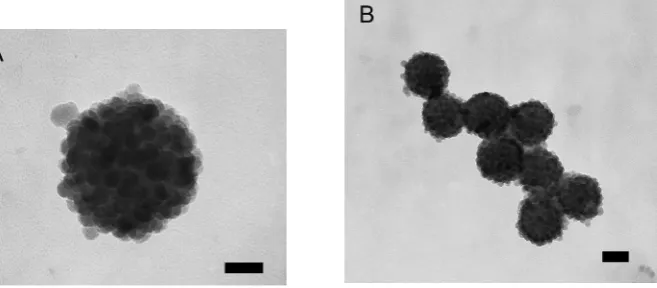
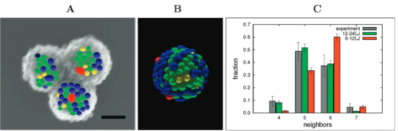
3.1 TEM images of colloidal silica armoured polystyrene latex particles. 30 3.2 Packing patterns of nanosized silica particles on the surface of polystyrene latex particles . . . 34
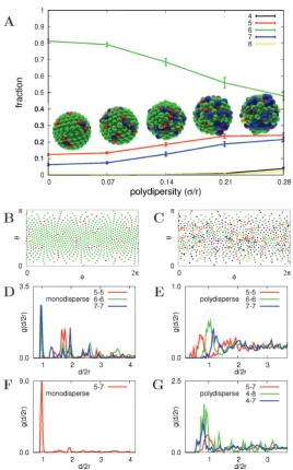
3.3 Theoretical results. . . 36
4.1 2D structures formed by a set of molecules with different angles between the bonding groups. . . 39
4.2 The three different hexagonal tiles considered in this work. . . 43
4.3 The solid phases obtained at low temperature. . . 46
4.4 Tile A, phase diagram at 50% coverage. . . 47
4.5 Tile A, parameters study. . . 48
4.6 Tile B, phase diagram at 50% coverage. . . 49
4.7 Tile B, parameters study. . . 50
4.8 Tile C, phase diagram at 50% coverage. . . 51
4.9 Tile C, parameters study. . . 52
4.10 Tile A: dvs. q phase diagram. . . 53
4.11 Tile B: d vs. q phase diagram. . . 54
4.12 Tile C: d vs. q scheme. . . 55
4.13 Tile B. The ratio hEPi E∞ is plotted againstq. . . 56
5.1 Actions . . . 63
5.2 Flowchart of the AB algorithm. . . 66
5.3 Set of particles used to test and develop the algorithm. . . 67
5.4 System energy vs simulation step (a) and vs CPU time (b). . . 69
5.5 Comparison of the relative improvements. . . 71
5.6 Final configurations. . . 72
5.7 Final configurations order. . . 73
5.8 Agent size evolution. . . 74
5.9 Evolution of several simulation parameters. . . 75
6.1 AB actions . . . 82
6.2 Link with TINKER. . . 84
6.3 TPA system. . . 85
6.4 Final energy. . . 86
6.5 CPU time comparison. . . 88
LIST OF FIGURES
6.6 TPA end simulation snapshots. . . 89
6.7 Correlation function g(r). . . 90
6.8 Simulation analysis. . . 91
6.9 Number of agent of each size. . . 91
6.10 Accepted moves. . . 93
6.11 Agents in end simulation snapshots. . . 94
6.12 AB end configuration energies . . . 95
6.13 Order parameters at constant density. . . 96
6.14 Order parameters at constant temperature. . . 97
6.15 TPA phase diagram. . . 98
A.1 AB, DA, MC comparison. . . 103
A.2 Phase diagrams of simple fluids. . . 104
A.3 Gay-Berne particles. . . 105
A.4 Colloidal particles. . . 106
A.5 Shrinking of the coexistence region in patchy particle’s phase diagram.107 S.1 Energy as a function of particle number. . . 111
S.2 Nearest neighbour distribution comparison between simulated and experimental data. . . 112
S.3 Tile A, density 0.10 . . . 113
S.4 Tile A, density 0.30 . . . 113
S.5 Tile A, density 0.50 . . . 113
S.6 Tile A, density 0.71 . . . 113
S.7 Tile B, density 0.10 . . . 114
S.8 Tile B, density 0.30 . . . 114
S.9 Tile B, density 0.50 . . . 114
S.10 Tile B, density 0.71 . . . 114
S.11 Tile C, density 0.10 . . . 115
S.12 Tile C, density 0.30 . . . 115
S.13 Tile C, density 0.50 . . . 115
S.14 Tile C, density 0.71 . . . 115
S.15 Parameters study. . . 117
S.16 Parameters study. . . 118
LIST OF TABLES
5.1 Simulation parameters and their optimised value. . . 76 S.1 Comparison between AB and MC simulations, simulation with 50
particles. . . 120
S.2 Average values of Emin, without single particle moves. . . 121
S.3 Average value of Emin, including single particles moves. . . 122
Acknowledgments
Amicitiae nostrae memoriam spero sempiternam fore. (Cicero)
In primis I gratefully acknowledge Dr. Alessandro Troisi, group leader and re-search supervisor of my postgraduate studies for his guidance, advice and feedback, and the collaborators of this thesis work: Catheline A. L. Colard and Dr. Ir. Stefan A. F. Bon, who performed the experiments reported in Chap. 3, both for the useful discussions on the studied system and for the fruitful collaboration; Dr. David L. Cheung, for suggestions, feedback and comments, in particular regarding Chap. 4. In addition, we thank Prof. Michael P. Allen for suggestions and inputs regarding the work of both Chap. 5 and Chap. 4.
We gratefully aknowledge the members of the Troisi Group directly involved in the project this thesis work is part of, namely “Modelling Techniques for Molec-ular Self-Assembly” funded by The Leverhulme Trust. We are grateful to Dr. Natalia Martsinovich for useful discussions on the theory of self-assembly of two-dimensional systems, explored in Chap. 4, with particular focus on the TPA system, studied in Chap. 6; Dr. Arijit Bhattacharyay, developer of the data augmentation algorithm (outlined in Appendix A.1), for fruitful discussions in the early stages of the development of the agent based program presented in Chap. 5; and Konrad Diwold, for useful discussion on object oriented programming.
We thanks the other members of the Troisi group: Daniel R. Jones for comments and discussions throughout the whole doctoral activity, and David P. McMahon for carefully proof-reading this thesis. In addition we are thankful to Dr. David Quigley, Dr. Rebecca Notmann, Dr. Christian Diedrich, for inputs and feedback, again throughout the whole doctoral activity.
Declaration and Inclusion of Material from a Prior Thesis
Part of the material contained in this thesis have been adapted from the fol-lowing publications, based on the author’s own thesis work:
Chapter 3
1. S. Fortuna, C. A. L. Colard, A. Troisi and S. A. F. Bon - Packing patterns of
silica nanoparticles on surfaces of armored polystyrene latex particles, Langmuir, 2009, 25 (21), pp 12399-12403.
Chapter 4
2. S. Fortuna, D. L. Cheung and A. Troisi -Hexagonal lattice model of the patterns
formed by hydrogen-bonded molecules on the surface, J. Phys. Chem. B, 2010, 114 (5), pp 18491858
Chapter 5
3. S. Fortuna and A. Troisi -An artificial intelligence approach for modeling
molec-ular self-assembly: Agent Based simulations of rigid molecules, J. Phys. Chem. B, 2009, 113 (29), pp 9877-9885.
4. S. Fortuna and A. Troisi -Agent Based algorithm for the study of molecular
self-organisation, Proceedings of the Sixth European Conference on Complex Systems, 2009, p24.
Chapter 6
5. S. Fortuna and A. Troisi - Agent based modelling for the 2D molecular
self-organization of realistic molecules, J. Phys. Chem. B, in press.
6. S. Fortuna and A. Troisi - Agent Based modelling of realistic molecules -
Pro-ceedings of the ECCS’10 European Conference on Complex Systems, 2010, in press.
In addition, Chapter 1 and Chapter 2 include material from all the cited sources, and the experimental work of Chapter 5 has been done by C. A. L. Colard, under the supervision of S. A. F. Bon.
The author also confirm that this thesis has not been submitted for a degree at another university.
Abstract
In this thesis we develop computational techniques for modelling molecular self-organisation. After a short review of the current nanotechnological applications of molecular assembly and the main problems encountered in modelling the self-organised behaviour of chemical systems, we introduce a set of methods, from both chemistry and complexity science, for the prediction of self-assembled structures, with particular focus on Monte Carlo (MC) based methods.
We apply the MC method to two systems of experimental interest. First we model the silica nanoparticles on the surface of spherical polystyrene latex droplets, synthesised by the S. Bon Group at the University of Warwick, as a set of soft spheres on a spherical surface, to study their packing patterns as a function of the broadening of the nanoparticle size distribution. Then we develop a hexago-nal lattice model for the study of the two-dimensiohexago-nal self-organisation of planar molecules capable of complementary interactions, to study their phase diagrams as a function of the strength of their complementary interactions and bonding motif. In both cases, the phases are characterised using a number of order parameters. We show that these simplified models are able to reproduce the experimental ob-servations.
Abbreviations
2D 2-Dimensional
3D 3-Dimensional
AB Agent Based
AI Artificial Intelligence
BH Basin-Hopping
CA Cellular Automata
CG Coarse-Grained
DA Data Augmentation
DFT Density Functional Theory
GA Genetic Algorithm
H-bond Hydrogen bond
IC Integrated Circuit
LJ Lennard-Jones
MC Monte Carlo
MD Molecular Dynamics
MM Molecular Mechanics
PBC Periodic Boundary Conditions
TPA terephthalic acid
1 INTRODUCTION
We will have to see that
we are the natural expressions of a deeper order.
(Stuart Kauffman, At Home in the Universe, 1995)
S
elf-organisation is the process by which a system increases its orderwithout an external driving force. The process of self-organisation is ubiquitous in nature: ants self-organise into colonies, people into soci-eties, cells into living beings. In chemistry, self-organisation generally refers to the formation of ordered molecular aggregates.
1.1 Self-Organisation in Chemistry
Self-organised structures in chemistry and biochemistry include cell membranes [1], virus capsids [2], and liquid crystals [3]. The units that form the self-assembled structures, or building blocks, can have any kind of shape (for example see Fig. 1.1(a)) and their size can range from that of a nanometer sized single molecule to nanoscale or microscale colloidal particles [4]. The driving forces that promote the self-assembly are the same non-covalent interactions of supramolecular chemistry [5, 6] such as Van der Waals, hydrogen bonds (H-bonds), electrostatics, and hydrophobic interactions.
Self-organised structures are thermodynamically stable, as they tend to adopt a configuration that corresponds to their thermodynamic minimum [8, 7]. In ad-dition, they are often kinetically labile, as they can rapidly explore the available configurational space. These two characteristics make the self-organising process a phenomenon that takes advantage of the reversibility of the non-bonded interac-tions which, under the right experimental condiinterac-tions, drives the system towards a unique product [9].
1.1 Self-Organisation in Chemistry
(a) (b)
Figure 1.1: (a) Possible shapes for liquid crystal building blocks, adapted from Ref.[3]. (b) Disconnectivity graph for an icosahedral shell composed of twelve pen-tagonal pyramids, figure adapted from Ref. [7]. Low-lying minima are illustrated near to their corresponding branches in the graph. The energy is in reduced units. This is a method to visualise in two dimensions the multidimensional free energy surface associated with the process. This particular structure for the disconnec-tivity graph identifies an efficient structure seeker, but in a typical simulation it is easy to get trapped in a relative minimum.
an efficient structure seeker, in which the global minimum of the potential energy surface (represented by the longer vertical line, in the graph of Fig. 1.1(b)) is kinetically accessible as there are no high energy barriers connecting the other local minima (represented by the other vertical lines). Wales also showed how a change in the building blocks can change the picture [10], generating other minima and/or making the global minimum less accessible.
Experimentally, it has been shown that changing the building blocks can even move the global minimum towards a different structure. In fact, as the shape or the strength of the interactions between building blocks changes, different assemblies
can emerge, which are often difficult to determine a priori. For example, the
structures shown in Fig. 1.2 are produced by the assembly of analogous molecules, each containing a rigid core with two hydrophilic groups at each end of the core, plus a hydrophobic side chain. In this example, the structure obtained by the self-assembly of a number of identical molecules, depends on the size of the side
1.1 Self-Organisation in Chemistry
Figure 1.2: Liquid-crystalline phases formed from amphiphilic molecules containing a rigid rod-like core and nonpolar lateral chains; A) smectic A, B) rectangular columnar, C) hexagonal columnar, D) laminated nematic, E) biaxial smectic A. Figure taken from Ref. [3].
chain [3]. The building blocks can also be modified by environmental changes, which leads to different structures. This characteristic is exploited in the study of dynamic materials [11] which can change their structure as a response to external stimuli (e.g. peptide based materials [12] and functionalised nanoparticles [13]).
In integrated circuit (IC) design [14], the self-assembly process constitutes an alternative to current lithographic techniques [15]. In fact, in IC fabrication there are benefits, such as higher speed and less energy consumed per computing func-tion, in decreasing the size of the electronic components [15]. It seems that the lithography based IC fabrication is approaching its limit and, even if the current chips printed by this technique are cheap, in the nanometer-scale self-assembly seems a cheaper alternative. Molecular electronics is being explored for high den-sity nanoelectronic devices [14, 16] where the open problem is how to wire the com-ponents together, or better, how to design comcom-ponents capable of self-assembly in the desired fashion. Current research is focused on nanotubes and nanowires [17], and on two-dimensional (2D) self-assembled ordered structures [18]. In particu-lar, the self-assembly of planar molecules on metallic surfaces is of great interest [19, 20, 21, 22] as several systems are capable of forming regular patterns, which in turn can be functionalised through the adsorption of other molecules [23, 24, 25].
1.2 Molecular Systems as Multiscale Complex Systems
are of particular interest considering that a large number of new drug candidates are not water soluble [26] and the carriers can be engineered such that they can assemble and disassemble as a function of the environmental conditions. In ad-dition, functionalised nanoparticles that can assemble or disassemble, or change their shapes in response to external stimuli can be used for biosensing [32], assay labelling [13], and bioimaging [33, 34].
Deeper knowledge of molecular self-assembly may even impact fields such as medicine, where understanding the process of the formation of amyloid fibres [35], associated with Alzheimer and spongiform encephalopathies, or virus capsids [2] may be a route towards new cures by inhibiting their assembly [36, 37].
In this context, the design of the necessary building blocks and the identifica-tion of the correct experimental condiidentifica-tions to obtain a structure with the desired properties are among the most challenging problems. In fact, even though we may have detailed knowledge of the interactions between the building blocks involved, considering a set of molecules and predicting the lowest energy configuration they can form is still challenging [38, 39]. Several methods have been developed for the study of molecular self-organisation, and in the following chapter we will overview them with particular focus on the Monte Carlo (MC) method, the basis of the majority of the work presented in this thesis. In the last two chapters we will propose an alternative approach for the study of molecular self-organising systems by treating them as complex systems.
1.2 Molecular Systems as Multiscale Complex Systems
There is no unique definition of complex systems [40], as this is an umbrella term used to describe systems in which a huge number of relationships can generate new patterns and whose collective behaviour is not easily derivable from the sum of its components behaviours. Self-organised systems, such as colonies, societies, living beings, and molecular aggregates are examples of complex systems and share a set of characteristics. All these systems are formed by identical, or similar, components. The components are related by a number of interactions, which can be either linear or nonlinear, simple or complicated. The sum of these interactions
leads to patterns, oremergent phenomena (i.e., the self-organisation itself). Given
the number of relationships involved, the behaviour of complex systems is difficult
to predict a priori. For example, looking at a cell we cannot predict a priori that
an ensemble of cells will produce a living being. In a similar fashion looking at a
molecule it is not possible to determinea priori which structure a set of molecules
will form. The observed patterns are in fact a consequence of thecooperative effects
1.3 Aim of this Work
acting among the components, which can contribute to enhance or elide a certain behaviour.
Characteristics that define a complex system, other than cooperative effects, are hierarchical organisationandmultiscale properties. Chemical systems possess these characteristics, as the process of self-organisation takes place at several length-scales and the molecules often come together in supramolecular structures that in turn self-assemble into larger structures. An example is the self-assembly of polypeptides known to form fibres [41, 42]. They interact in the direction of the fibre elongation through several H-bonds and on the other directions thanks to Van der Waals interactions. The polypeptides first form unidimensional fibrils and only at longer timescales will the fibrils self-assemble into fibres. The driving force of the fibre formation is the sum of the Van der Waals interactions acting between the sides of the molecules which is the result of the cooperative effects between the polypeptides. We therefore observe the formation of hierarchical structures at different timescales and different length-scales. A hierarchical spatial organisation is by definition a multiscale process.
We therefore propose in this work that self-organising chemical systems can be studied with the tools of complexity science.
1.3 Aim of this Work
The aim of this thesis is to bind together concepts and techniques from complex-ity science with the traditional computational chemistry tools in order to study molecular self-organisation.
The main aspect imported from complexity science regards the identification of the simplest features a system needs to possess in order to be able to express a determined behaviour. In this context, we will assume that self-organisation is an emergent phenomenon due to the interactions among a collection of particles and find the minimum number of relations able to give a certain pattern. In self-assembly this can be achieved either (i) with a minimal model to represent the system under investigation and/or (ii) with a minimal representation of its dynamics. In this thesis we will investigate both of these aspects.
1.4 Thesis Outline
Then we will develop a hexagonal lattice model, for the study of the 2D self-assembly of planar molecules on surfaces. We will show that this symplified model is able to reproduce many of the patterns encountered in experimental systems.
Finally, we will move onto the key aspect of this thesis work, by introducing a new modelling paradigm in the field of molecular simulations. This will be done through the implementation of a rule-based algorithm, namely an Agent Based (AB) algorithm, first proposed as a lattice algorithm [43]. First the AB algorithm will be developed for the study of off-lattice systems, then, in order to be able to recover the system-specific knowledge, we will link the AB algorithm to an available code to calculate properties of a realistic system.
1.4 Thesis Outline
This thesis is organised as follows: in Chap. 2 we will overview models and methods that can be used for the study of molecular self-organisation, with particular focus on the MC method. The latter will be used in Chap. 3 to study the packing patterns of spherical silica nanoparticles on the surface of spherical polystyrene latex droplets, and in Chap. 4 to study the 2D patterns formed by planar molecules capable of complementary interactions on metallic surfaces, with an hexagonal lattice model. In Chap. 5 we will introduce our AB model for the study of molecular self-organisation of a set of idealised shapes, and in Chap. 6 we will extend the AB model for the study of realistic system. Chap. 7 concludes the thesis.
2 MODELLING TECHNIQUES AND THEORETICAL BACKGROUND
.. it is requisite that its parts mutually depend upon each other
both as to their form and their combination,
and so produce a whole by their own causality ..
(Immanuel Kant, The Critique of Judgement, 1892)
W
e introduce herethe background knowledge for the modelling ofself-assembling chemical systems. We first discuss the model systems used to describe the building blocks of the molecular self-organisation, then, after some basic definitions of statistical physics, we will briefly review simulation methods used both in chemistry and in complexity science.
2.1 Model Systems
The building blocks of molecular self-assembly usually consist of molecules contain-ing between 10 and 1000 atoms. They can be defined at many levels of physical accuracy: as occupied lattice sites, as idealised shapes, or as point masses (atoms) held together by suitable interatomic potentials. Simple lattice models have been very useful, before the advent of the computers, to calculate analytically the first phase diagrams [44]. The advent of computers however, together with the increase of available computational power, allowed for the study of more complicated sys-tems: from simple systems composed of spherical particles, up to detailed atomistic models. In this thesis, we will treat the building blocks as rigid bodies, without internal degrees of freedom, focusing our attention on the intermolecular forces driving the self-assembly process.
2.1.1 Lattice Models
2.1 Model Systems
(a) (b) (c) (d)
Figure 2.1: (a) Gas-lattice model: occupied sites are black and empty sites are white. (b) Hexagonal particles with two charged edges, figure adapted from Ref.[45]. (c) Tetromino particles occupy multiple lattice sites, in this case each site can be neutral (red), positively (blue) or negatively (black) charged, figure adapted from Ref.[43]. (d) Lattice polymers in random coil (top) and polycrys-talline (bottom) conformations.
study phase transitions analytically [47]. In a lattice gas model, particles are represented as occupied sites on a lattice, often a square lattice as in Fig. 2.1(a). The system is described by a Hamiltonian that takes into account the Van der Waals interactions between particles:
H =−²X
hi,ji
ninj (2.1)
where ² is the interaction strength, ni = 0 if the cell i is empty, ni = 1 if it is
occupied, and the summation is taken over adjacent cells. The lattice gas model, derived from the Ising model [46] used for the study of ferromagnetism and in which
each lattice site can assume the states si = ±12, can be converted into the Ising
model by the linear transformation ni = si+12 . Therefore the model is isomorphic
to the Ising model, and all the results for the Ising model also apply to the lattice gas model. The Ising model, proposed and studied analytically in one dimension by Ising in 1925 [48] and extended to 2 dimensions by Onsanger in 1944 [49], is the first of a small set of analytically solvable models for the study of phase transitions [44].
Among the extensions of the simple lattice gas model, there are Potts models [50] in which the lattice sites can assume a number of states larger than two, and models in which the particles have an internal structure. Examples of the latter include Ice-Type models on the square lattice [44], the Poker Chip model on
2.1 Model Systems
-1 -0.8 -0.6 -0.4 -0.20 0.2 0.4 0.6
0.5 1 1.5 2 2.5 3 Eij
rij
LJ LJ+Coulomb LJ + Yukawa
1
(a) (b) (c) (d)
Figure 2.2: (a) Spherically symmetric potentials. (b) Gay-Berne particles: elon-gated (top) and discotic (bottom). (c) Two amphiphilic particles with hydrophilic headgroups (red) and hydrophobic tails (blue) to model micelle formation, taken from Ref. [61]. (d) Model with distinguishable particles, taken from Ref. [62].
the hexagonal lattice [51], and the model we will introduce in Chap. 4 where the hexagonal building blocks (Fig. 2.1(b)) interact with a Hamiltonian able to describe both Van der Waals interactions and directional H-bonds. It is also possible to
include long range interactions, for instance a dipolar interactionHD =DPij nri3nj
ij as in Ref. [52]. Models of this type are rarely analytically solvable.
2.1 Model Systems
2.1.2 Rigid-Soft Models
In the continuum space, the sphere is the simplest particle model we can think of.
Simple impenetrable spheres that cannot overlap are described by a hard sphere
potential [63]:
Ehard
ij =
(
0 if |rij| ≥ri+rj
∞ if |rij|< ri+rj (2.2)
where rij is the distance between the centers of the spheres with radii ri and rj
respectively. This was one of the first systems studied using computer simulations by the pioneers of the field [64, 65, 66, 67].
Another system of interest, first approached in the paper of Rosenbluth and Rosenbluth [65], is a system composed of soft spheres described by a Lennard-Jones (LJ) like potential (Fig. 2.2(a)) of the form:
ELJα−2α
ij =²0
·µr
eq
rij
¶2α
−2·
µr
eq
rij
¶α¸
(2.3)
where²0 is the depth of the potential well,req is the equilibrium distance between
them, andαis a parameter describing the “softness” of the potential. Large values
of α give a harder potential, in which particles are less likely to compenetrate,
and viceversa. For example, the argon atoms described by a LJ potential with
α = 6 have very soft boundaries and this is consistent with the observation that
the boundaries are defined by their electron clouds and allow for compenetration, on the other hand the silica nanoparticles of Chap. 3, being composed of several
atoms, are better described with a harder potential (for exampleα = 12).
Charges can be included by addition of a Coulomb term:
EC
ij = 41π²qriqj
ij (2.4)
whereqi and qj are the charges of each particle and ²is the electrical permittivity.
Alternatively, as in the case of colloidal particles, it is possible to describe the elec-trostatic interactions through a Yukawa potential (or screened Coulomb potential) [68, 69]:
EYukawa
ij = A·exp((r −rij/ξ)
ij/ξ) (2.5)
whereξ is the screening length parameter, and A= qiqj
4π². The screening parameter
takes into account the fact that colloidal particles often have surface charges and are surrounded by electrolytes which screen the effective Coulomb interactions between colloids.
2.1 Model Systems
Hydrophobic terms are more difficult to include, as these interactions are due to the rearrangement of water molecules and H-bonds as two hydrophobic molecules come together. However, they can be modelled for example with a potential of the
formEijhp =−γ−rij/λ, whereγ is a surface tension constant, andλthe range of the
hydrophobic interaction [61].
If the building blocks are not spherically symmetric and anisotropic, as with liquid crystals, it is possible to use the Gay-Berne potential [70]:
EGB ij = 4²
"
½ σ
xy
rij −σ+σxy
¾12
−
½ σ
xy
rij −σ+σxy
¾6#
(2.6)
where both ² and σ depends first of all on the orientation of the particles, and
their separation vector. In addition, Gay-Berne particles interact with different
strengths in the x, y plane with respect to the z direction, and this is taken into
account in the functional form of ², and the aspect ratio between the two can be
adjusted to give either elongated (Fig. 2.2(d), top) or discotic (Fig. 2.2(d), bottom)
particles. The latter aspect is taken into account by the form of σ which depends
on the length and breadth σxy of the particles.
Alternatively, it is possible to describe a non spherical building block using
several LJ spheres. For example Tsonchev et al. [61] studied the self-assembly
of amphiphilic molecules for the study of micelle formation, modelling them as rigid cones composed of spheres which interact with a hydrophobic term plus a Coulombic term (Fig. 2.2(c)). Sciortino [71] studied gel formation of systems com-posed of patchy particles, and LJ spheres with attractive spots on their surface. Zhang and Glotzer [62] studied several systems of particles composed of different
LJ spheres each characterised by a different value of ²0, as shown in Fig. 2.2(d),
to understand the effect of the shape and of the different interaction strengths on the self-assembled structures. In Chap. 6 we will test our algorithm on a set of three-dimensional (3D) tetromino-like shapes composed of different arrangements of LJ spheres which can be neutral, positively, or negatively charged.
2.1 Model Systems
Figure 2.3: Force-field contributions. Taken from Ref. [72].
2.1.3 Molecular Mechanics Based Models
Molecular mechanics (MM) models rely on a classical treatment of particle-particle interactions. Molecules in MM are represented as particles connected by a set of “springs”, which represent the chemical bonds. Each particle can represent either a single atom, as in atomistic models, or a group of atoms, as in CG models.
The interaction between the particles are described by a force-field [72], which
typically includes intramolecular terms such as bending, stretching, and torsions (see Fig. 2.3), and intermolecular terms, such as Van der Waals, electrostatics, and H-bonding.
The bonding energy is well described by a Morse potential EMorse(l) =De[1−
e−a(l−l0)]2 with D
e depth of the energy minimum, a = ωpµ/2De where ω is the
frequency of the bond vibration,µis the reduced mass, l0 the average bond length,
and l the current length. However, as it requires three parameters, usually the
harmonic potential is used instead, which requires only two parameters:
Estretching(l) = k2l(l−l0)2 (2.7)
This correspond to the first nonzero term of a Taylor expansion around the equi-librium configuration. Additional terms of the expansion, such as cubic or higher terms, can be included to better reproduce the Morse curve. The bond-angle energy can be computed as:
Ebending(θ) = k2θ(θ−θ0)2 (2.8)
where kθ is the harmonic force constant, θ0 is the equilibrium angle between 3
particles, θ the current angle. As for the stretching energy, higher order terms can
2.1 Model Systems
also be included. The torsional energy can be expressed as:
Etorsion(ω) =
N X
n=1
Vn
2 (1 + cos(nω−γ)) (2.9)
where Vn gives an indication of the height of the energy barriers between the n
minima, γ is the phase factor which determines the position of the energy minima,
and the number of terms N can be adjusted to take into account the number of
expected minima. In addition other terms can be included, such as out-of-plane bendings and cross-terms to couple two degrees of freedom [72].
The basic functional form of the intermolecular potential is usually based either on a LJ potential (described in the previous section) or on a Buckingham potential
Ebuckingham=Ae−Br−Cr−6 (2.10)
which has a softer repulsive component with respect to the LJ potential. Elec-trostatic contributions can be taken into account as charge-charge interactions, through a Coulomb term as in Eq. 2.4, or as bond dipoles. In addition, other terms can be included such as H-bonds energies, or quadrupoles moments.
All the functions used to describe both intra- and intermolecular energies, de-pend on a set of parameters that can be either obtained from quantum mechanical calculations or from experimental data. Functions together with their parameter set completely define a force-field. In the case of atomistic models, well established force-fields include MM2/MM3 [73, 74] first proposed by Allinger in 1977 for small organic molecules, and Amber [75, 76] proposed by by Weiner and co-workers in 1984 [75] for proteins and nucleic acids.
If a full atomistic representation is not feasible, it is possible to coarse-grain
the system [77, 78], considering groups of atoms as a single unit. This allows the study of larger systems at longer timescales. The parameterisation of CG
models is usually performed via the comparison with atomistic models. Examples
of CG potentials include the MARTINI potential [79], for the study of amphiphilic molecules where, on average, four heavy atoms are represented by a single CG unit. Other CG models are often used to describe proteins [80], in which each amino acid can be represented as a particle (or bead), or polymers [81], in which every repetitive unit is represented as a bead. In both cases, side chains can be taken into consideration as additional beads.
sec-2.2 Some Statistical Mechanics Definitions
tion, as they can be derived from and mapped back to an atomistic representation [81]. The possibility of a mapping between different levels of approximation is a key feature of the multiscale models that will be introduced in Sec. 2.3.3.
2.2 Some Statistical Mechanics Definitions
A system at equilibrium can be in one of many possible microstatess. A property
Q will assume a value Q(s), depending on the current microstate of the system.
However, experimentally we measure Q in a finite time interval τ performing a
time average:
Qexp = 1τ
Z τ
0 Q[s(t)]dt (2.11)
as the microstate of a system s(t) can change over the observation time τ. In
simulations time is discrete, and for molecular dynamics (MD) simulations (see Sec. 2.3.1) we can measure the same property as:
QMD =hQit= n∆1t n X
i=1
Q[s(i∆t)] (2.12)
As this is not always possible nor necessary, we make use of the ergodic theorem
that states that, at the thermodynamical equilibrium, averages taken over time on a given system are the same as averages taken over many replicas of the same system with the same macroscopic characteristics. The replicas of the system under
investigation with similar macroscopic parameters form a statistical ensemble. A
number of ensembles are known from statistical thermodynamics [82, 83] and are
commonly used: (i) the microcanonical ensemble or NV E ensemble, in which all
the systems have the same volume V, the same number of particles N, and are
thermally isolated with the same total energy E; (ii) the canonical ensemble or
NV T ensemble, in which all the systems are in thermal equilibrium with a large
heat reservoir or heat bath large enough to keep the temperature T constant, and
(iii) the grand canonical ensemble, which is in thermal contact with a bath and allows for exchange of particles.
The ergodic theorem is of great practical use, as it allows us to run simulations
on a numberM of replicas of a system, and average over observations taken at the
same simulation timet0:
hQiM = M1 M X
m=0
Q[sm(t0)] (2.13)
2.3 Simulation Methods in Chemistry
In addition, given a statistical ensemble, if we define ps as the probability of a
replica being in a certain states, we can average over states writing:
Q=hQis= X
s
Qsps (2.14)
Eq. 2.14 is the form used in MC simulations (Sec.2.3.2).
2.3 Simulation Methods in Chemistry
Once the building block representation has been chosen, it is necessary to choose a theoretical method to describe the system properties. Several methods have been developed to study molecular systems and, traditionally, each simulation method is bound to a unique time/length-scale, as shown in Fig. 2.4. At the extreme of small and large scales there are methods that do not rely on the previously intro-duced models: quantum chemical calculations and continuum models. At small time/length-scales quantum chemical studies have been successfully used to iden-tify the lowest energy dimers, trimers, and tetramers thought to be the supramolec-ular building blocks of larger structures [84, 85, 86]. At the other extreme, where very large time/length-scales prevail with respect to the atomic constituents, as in fluid dynamics [87] or the simulation of mechanical properties, continuous models can be employed. Between the two scales there are the two methods used for the study of self-organisation of ensembles of molecules: MD and MC.
In this thesis, we will mainly focus on MC-based methods. However, for com-pleteness, in this section we will also briefly overview the MD method.
2.3.1 Deterministic Methods: Molecular Dynamics
The MD simulation method [88] is based on Newton’s second law or the equation
of motion, ~Fi = mi~ai, where ~Fi is the force exerted on a particle i with mass
mi, and ~ai is its acceleration. The force can be expressed as the gradient of the
potential energy (E): ~Fi =−∇~iE, whereE is represented by one of the force-fields
introduced in Sec. 2.1. Integration of the equations of motion yields a trajectory that describes the positions and velocities of the particles as they vary with time. From this trajectory, the average values of properties can be determined through Eq. 2.12. The method is deterministic: once the positions and velocities of each atom are known, the state of the system can be predicted at any time in the future or the past.
2.3 Simulation Methods in Chemistry
Figure 2.4: Simulation methods in chemistry. On the x-axis the system length-scale, on the y-axis the timescale. From this plot it is possible to see that every technique is bound to a unique time/length-scale. Taken from Ref. [81].
time is explicitly included, allowing for the calculation of time-dependent proper-ties. Usually MD simulations relax fast towards the nearest local minima and are not suitable for overcoming high energy barriers between configurations, because of the very small time/length-scales they can reach [89]. However, if the target configuration of a system is known, they are a useful tool to study its equilibrium behaviour.
Many implementations of the method have been developed in order to escape the local energy minima, and therefore reduce the computational time by arti-ficially speeding up the exploration of the configurational space. Strategies like hyperdynamics [90], temperature accelerated methods [91], metadynamics [92], activation-relaxation techniques [93, 94] might be used to overcome this problem. For example in hyperdynamics [90] a bias potential can be used to raise the energy of the system in regions other than that of the transition state, but this method has never been used for cluster formation or self-assembly. Similarly the
2.3 Simulation Methods in Chemistry
ture accelerated method, in which part of the simulation is carried out at higher temperature, has not been used for these scopes. Metadynamics [92] is one of the methods of choice to study crystal nucleation [95, 96], as with this method it is possible to fill the explored potential wells with Gaussians [97], in order to flatten the surface and explore the whole configurational space. This method has been
suc-cessfully used by Quigleyet al. to study water [95] and calcite nucleation [96]. The
activation-relaxation technique [93, 94] allows the system to explore neighbouring local minima by deforming the system (activation) to let it escape a local minimum and then the system is pushed into an adjacent minimum (relaxation). Mousseau explored the early stages of fibre formation with an activation relaxation technique [98] observing, for short sequences, the formation of parallel dimers, trimers and hexamers.
MD methods are therefore implemented for the detailed study of small groups of molecules, making it possible to explore the transition steps in the very first stages of molecular self-organisation, but to study systems composed of hundreds of molecules they are limited by the short timescales and long computational time required.
2.3.2 Stochastic Methods: Monte Carlo
The MC method is a stochastic method, first proposed by Ulam and Metropolis in 1949 [99] to study systems composed of a large but finite number of particles. The idea behind the MC method [64, 83, 88] is that, in order to estimate Eq. 2.14
without a priori knowledge of the functional form of ps, it is possible to consider
the possible states of a system at the equilibrium as areversible Markov chain, and
estimate Q as:
QM = M1 M X
i
Qi (2.15)
where the average is taken over a Markov chain of lengthM.
A Markov chain is a chain of states in which the transition probabilityP(s0 →s)
from a state s0 to a state s depends only on s0, allowing one to write the master
equation of the system as:
dps
dt =
X
s0 ·
ps0(t)P(s0 →s)−ps(t)P(s→s0) ¸
(2.16)
2.3 Simulation Methods in Chemistry
respectively. At equilibrium, the steady state approximation (dps
dt = 0) applies:
X
s0
P(s→s0)p
s = X
s0
P(s0 →s)p
s0 (2.17)
and, in order to eliminate limit cycles, in which the system explores cyclically a set of states without necessarily exploring the whole state space, the detailed balance should be satisfied:
P(s→s0)p
s =P(s0 →s)ps0 (2.18)
which can be rewritten as:
P(s→s0)
P(s0 →s) =
ps0
ps (2.19)
In 1902, Gibbs showed that a system in thermal equilibrium with a reservoir, in
theNV T ensemble, can be in one of several possible microstatesswith probability:
ps = Z1e−Es/kBT (2.20)
where Es is the energy associated with the microstate s, kB is the Boltzmann
constant, T is the system temperature, and Z is the partition function of the
system. The partition function can then be derived as a normalisation constant,
given that P
sps = 1 we get:
Z =X s
e−Es/kBT (2.21)
combining Eq. 2.19, 2.20 and 2.21, the transition probability becomes:
P(s→s0)
P(s0 →s) =e
−Es0 −Es
kBT (2.22)
Given the transition probabilities, it is then possible to choose any algorithm to build up the chain of states. We can therefore break up the transition probabilities
into two terms, separating the probability g(s → s0) of proposing a new
configu-ration s0 from the probability of accepting the proposed configuration A(s → s0),
and rewrite Eq. 2.22 as follows:
P(s→s0)
P(s0 →s) =
g(s→s0)
g(s0 →s)·
A(s→s0)
A(s0 →s) (2.23)
In the Metropolis algorithm, one sets g(s → s0) = g(s0 →s) (i.e., the probability
of proposing a move is the same for opposite moves) and the relation between the
2.3 Simulation Methods in Chemistry
acceptance probabilities must be:
A(s→s0) = A(s0 →s)e−Es0 −Es
kBT (2.24)
with 0 ≤ A(s → s0) ≤ 1 and 0 ≤ A(s0 → s) ≤ 1, as they are probabilities. As
we want to maximise the acceptance ratio, it is convenient to give the larger of the two acceptance probabilities the value 1 and adjust the other. The Metropolis acceptance probability is therefore:
A(s →s0) = min[1, e−Es0 −Es
kBT ] (2.25)
first tested in 1953 for the simulation of a set of 224 rigid spheres in two-dimensions [64].
In general, the Metropolis sampling scheme can be used either for off-lattice and lattice models, and it is useful for systems that do not present high energy barriers between states [100, 101]. For example, in this thesis, the method will be applied to simple systems in both Chap. 3 and Chap. 4, to simulate silica nanoparticles on the surface of a polymeric nanodroplet, as a set of LJ spheres on a spherical surface, and H-bonded molecular networks on a metallic surface, with a hexagonal lattice model, respectively. The Metropolis MC scheme works well for simple systems and it has been proven that systems simulated with MC will converge to the Boltzmann distribution, but the number of simulation steps required to reach
equilibrium cannot be determined a priori [102], and the simulations can take a
very long time. However, it is possible to improve MC simulations for the study of self-assembled structures in several ways.
The first simplest modification of the MC method for structure prediction is simulated annealing [83, 103], inspired by the analogy with physical annealing, where a system, initially at a high temperature disordered state, is slowly cooled down becoming more and more ordered. This is achieved in the MC simulation by
varying the system temperatureT according to a cooling schedule. In theannealed
MC, at the beginning of the simulation the acceptance probabilityA(s→s0) is very
high, leading the system to explore many different configurations by escaping from
local minima, then, as the simulation evolves the probability A(s → s0) becomes
2.3 Simulation Methods in Chemistry
Alternative techniques of global optimisation in molecular systems include basin-hopping (BH) [7], replica exchange (also known as parallel tempering [104]), and the introduction of multiple particles moves into the MC algorithm. In BH [7] a new configuration is generated, its energy is minimised, and is then accepted or rejected based on the Metropolis criterion. In this way the real potential en-ergy surface is transformed into a set of plateaus (= basins) where the barri-ers between local minima are flattened out. In replica exchange [104, 105], two or more parallel simulations are run at different temperatures and, occasionally, configurations are swapped between the simulations with a probability given by
Pa,bswap = min
·
1,exph− Eb−Ea
kB(Ta−Tb)
i¸
where Ea is the energy of the system a at
tem-perature Ta and Eb is the energy of the system b at temperature Tb.
Multiple particle moves can be introduced in the algorithm defining groups of particles both on geometric [106] or energetic [107, 108] considerations. For example, the algorithm developed by Liu [106] is based on geometric considerations as follows: at every simulation step a pivot point is chosen at random, and a random particle is moved by reflection with respect to the pivot point, when this correspond to an overlap with other particles the other particles are moved with the same method. This is repeated until no overlap occurs anymore. On the other hand, the algorithm implemented by Bhattacharyay [107], the data augmentation (DA) algorithm, is based on energetic considerations: two particles are considered forming a cluster if they are bonded, and they are bonded with a certain probability that depends on their interaction energy. At every DA step, a particle is chosen, a cluster is defined, and it is moved. The cluster move is then accepted or rejected with a modified acceptance probability (see Appendix A.1), in order to keep the detailed balance. Among the algorithms capable of group moves, the DA algorithm [107, 108] is the one with which we will compare the algorithm presented in Chap. 5. The introduction of group moves in a MC simulation scheme is a key aspect to reach faster convergence [107, 108], as this allows for multiscale moves capable of escaping local energy minima. This aspect will be included in the AB algorithm of Chap. 5 and Chap. 6.
2.3.3 Multiscale Methods
According to Peter and Kremer [81], the term multiscale simulation “refers to methods where different simulation hierarchies are combined and linked to obtain an approach that simultaneously addresses phenomena or properties of a given system at several levels of resolution and consequently on several time- and
2.4 Simulation Methods in Complexity Science
scales.”
The coexistence of several simulation hierarchies can be achieved by introducing multiscale moves into a MC algorithm, as shown in the previous section where we introduced MC algorithms capable of binding different length-scales thanks to group moves. Another way to introduce group moves into a MC algorithm, is to mix it with MD in a hybrid scheme as with mixed MC-stochastic dynamics methods [109]. In this algorithm MC steps are alternated with stochastic dynamics steps, in order to perform group moves, thanks to MD, and reach longer timescales than MD alone without losing the microscopic detail. Even though the possibility of multiscale moves is a key element of the algorithms of Chap. 5 and Chap. 6, the implementation of another aspect of the multiscale modelling is a parallel field of open research: the implementation of strategies to combine different levels of resolution of the system under examination.
The possibility of multiple resolutions currently involves a sequence of simu-lations going from detailed simusimu-lations (e.g. MD with atomistic models) towards CG simulations, in order to extend the approachable time/length-scales with MD simulations. At every step of the procedure, the results of the detailed simula-tion are used to parametrise the next level of descripsimula-tion and, eventually, build up a mapping between the two in order to recollect the microscopic details from the mesoscopic simulations. Procedures of this type have been used for the study of polymers [110, 111]. Hybrid simulations are also used, in which atomistic de-tails are considered for the interesting portions of the system and the rest of the system is described with CG models. In this framework, the adaptive resolution scheme (AdResS), developed by Praprotnik [112], is particularly promising: this is a method in which molecules can enter and exit an atomistic region and adapt their description to the region in which they reside (see Fig. 2.5). However, currently these approaches have not been used for the study of self-organising systems, as they are very preliminary works.
In this thesis, we argue that the way to swap easily among scales with little computational effort relies on rule based models, in particular AB models, de-scribed in the next section. We believe that the inclusion of features like adaptive resolution schemes, might form part of the future development of the AB algorithm developed in Chap. 5 and Chap. 6.
2.4 Simulation Methods in Complexity Science
configura-2.4 Simulation Methods in Complexity Science
Figure 2.5: Adaptive resolution scheme. Molecules adapt their resolution level “on the fly”, water molecules can go from a CG description (left) to an atomistic one
(right) and viceversa. Figure taken from Ref. [112].
tions; (ii) sampling from the ensemble of configurations available to the system at equilibrium; (iii) finding physical pathways between stable or metastable states, on either the energy or free energy landscape. In this thesis we are mainly concerned with generating low energy configurations and sampling the ensemble configura-tions of a system at equilibrium, neglecting the last aspect. As a sampling scheme we will use the Metropolis MC scheme throughout all the thesis. However, when generating low energy configurations, regardless if the evolution of coordinates towards those configurations is unphysical, we can take advantage of a number
of other methods. Examples includes artificial intelligence (AI) based methods,
e.g. genetic algorithms (GA), orrule based models, such as cellular automata (CA)
or AB models.
2.4.1 Genetic Algorithms
A GA is a “search techniques based on the principles of natural evolution” [113, 114, 115] and it is generally used as a global optimiser. The parameters to be optimised are collected into a vector. In a GA every vector is considered an individual, part of apopulation, that represents a trial solution of the problem. The population evolves following bio-inspired rules as follows: at every simulation step (or generation) each
individual is ranked according to a fitness function, which quantifies the quality
of the trial solution, and then selected or discarded following tournament rules in order to create a new population. The new population is created either by a crossover operation, in which two individuals selected from the previous generation
are mixed to generateoffsprings, or bymutation, in which an offspring is created by
a random modification of an individual of the previous generation. The offsprings are then the new starting population for the next simulation step. This model has
2.4 Simulation Methods in Complexity Science
Figure 2.6: One-dimensional CA; the time step increases from left to right and successive time-steps are shown on successive columns; the 1-cells are represented by stars, the 0-cells by blank. Figure adapted from Ref. [120].
been successfully used for cluster geometry optimisation [113], where each cluster corresponds to an individual that, at every simulation step, is randomly rotated and cut into two parts. Two randomly selected parts belonging to two different clusters, are then merged into an offspring, and the offspring are ranked (in this case their fitness is related to their internal energy) and selected with a Metropolis acceptance probability (as Eq. 2.25), in order to pass to the next generation. The method has also been used for crystal structure prediction [116], protein folding [117], and self-assembly [118].
2.4.2 Cellular Automata
CA are lattice rule based models [119], in which each cell can be in one of a finite number of states and can change state following a set of rules based on its own state and the states of the neighboring cells, called the neighbourhood. At each simulation step, the rules are applied to the whole grid and a new generation is created.
For example Fig. 2.6 shows a one-dimensional two-state CA that presents self-similarity and fractal structure [120]. The updating rule is very simple: when the two neighbouring sites have the same value, the site assumes the value 0 indepen-dently of its current state, otherwise it assumes the value 1. Analogous patterns can emerge also in 2D CA from a few nonzero initial cells [121]. Wolfram [120] proposed that this and similar models can be interpreted as a crystal growth from an initial seed.
2.4 Simulation Methods in Complexity Science
height of a random point is increased by unity. If the height at one point exceeds a critical value, then a topping event occurs, the height of the point is reduced by 4 units and the height of the 4 neighbouring sites is increased by one. If any of the neighbours is now unstable, the process continues until none of the points of the system exceed the critical value. The size distribution of the avalanches follows a power law distribution, proving that a small perturbation (i.e., adding one single grain to a sandpile) can sometimes lead to very large avalanches. This model has been generalised to represent earthquakes [123] or economic events [124].
CA also have applications in biology, as in the study of population dynamics[125], and in chemistry [126, 127, 128, 129] as it has been extensively proven that the rules are particularly suitable as an alternative to partial differential equation models. CA have been used in chemistry to study reaction kinetics [126], recrystallisation [127], particle nucleation [128] and fluctuations in cluster formation [129]. The ca-pabilities of this modelling paradigm are obviously limited by its discrete nature.
2.4.3 Rule Based Artificial Intelligence: Agents
AB models are rule based models based on the collective behaviour of a set of
agents. By definition, “an agent is a computer system capable of exchanging
in-formation with other agents and its environment, taking decisions and performing autonomous actions” [130]. AB models have traditionally been used in fields like economics [124] or sociology [122, 131] to model the behaviour of complex systems such as stock markets and societies. For example, to model the stock market [124], agents can be identified with traders and, to model social phenomena, like the emergence of hierarchy in the society [131], agents can be identified as warriors. Agents share a set of characteristics: (i) they have a a set of properties, such as a position in space, a pot of money if they are traders, or an amount of “power” if they are warriors [131]; (ii) they evolve in time through a set of actions, for exam-ple buying and selling stocks or fighting; (iii) they are goal-oriented, for examexam-ple traders want to maximise their income and warriors want to maximise their power. In order to reach their goal, agents will decide which action to perform basing their decision on a set of conditions. Conditions and actions form the rules of an AB
model. In general, the AB rules are: (i) nonlinear, as they can contain if-then
conditions or more complicated algorithmic decisions; (ii) local, because only the
local environment may be considered by the agent before undertaking an action;
and (iii) adaptive, allowing the rules to evolve in time, to best suit the goal of the
simulation. In particular, the adaptation is a characteristic of the AB rules not
2.4 Simulation Methods in Complexity Science
present in the CA ones. The adaptability of the rules can have a great effect on the performance of the algorithm, leading it to reach the expected goal with less computational effort, such as less memory storage and/or computing time.
AB models have been introduced in chemistry [132, 133, 134, 43, 135], under the assumption that chemical systems are complex systems and it is therefore possible to describe their complex dynamics with a set of rules. For example, Cartwright et al. [132, 133] modelled the enantiomeric crystallisation of molecules letting each agent correspond to a nucleation site of L or D handedness. Each agent is then put into a flux, to study the effect of the stirring on the growing crystals. The model is based on four simple rules: new agents can appear both as new nucleation sites (with random handedness), or derive from an already existing nucleus (therefore with its same handedness), they can then either grow or dissolve. This model shows that, in agreement with the experiments [136], crystals under stirring conditions are all D or L. Bradford and Dill studied the the self-organisation of proteins [134]. In their model, proteins acting as catalysts are identified as agents able to move in space, with moves biased such that each agent is driven towards a region of space rich in its reactant. The end simulation result is that proteins tend to self-assemble into multicomponent aggregates in order to catalyse all the reactions of a chain. Troisi, Wong, and Ratner [43] studied the packing of a set of molecules to find their lowest energy configuration. In their model, an agent is identified with a shape or a group of shapes on a square lattice. At the begginning of the simulation each agent coincides with a rigid shape and, as the simulation proceeds, the agent evolves to represent stable portions of the system. Each agent evolves due to three actions:
move to a new position of the lattice, merge with another agent, and split into
3 MONTE CARLO SIMULATION OF POLYDISPERSE SPHERES ON
A SPHERICAL SURFACE
There is geometry in the humming of the strings,
there is music in the spacing of the spheres.
(Pythagoras, 6th.century BC)
I
n collaboration with the Bon Group, we studied the packingpat-tern of silica nanoparticles on the surface of spherical polystyrene la-tex droplets with MC simulations. The experimental system has been modelled as a set of interacting spheres on a spherical surface. The information supplied by this model has been complementary to the experimental data. We study the effect of the polydispersity of the spherical nanoparticles on the self-assembled structure. We show that broadening of the nanoparticle size distribution has pronounced effects on the self-assembled equilibrium packing structures, with the original 12-point dislocations or grain-boundary scars gradually fading out.
3.1 The Sphere Packing Problem
Packing patterns of identical and non-identical spherical and discotic objects on curved surfaces are often encountered in nature and science. Examples include C60 fullerenes [137, 138], 13-atom cuboctahedral metal clusters [139], S-layer pro-teins on outer cell membranes [140] which are all formed by the self-assembly of identical building blocks, and the lenses on insect eyes, biomineralized shells on coccolithophorids [141], solid-stabilised emulsion droplets [142] and bubbles [143], made of building blocks of different sizes.
It is well known that the maximum packing density of a single layer of spheres of identical size in an infinite 2D flat plane is achieved when they are arranged into a hexagonal lattice, with each of the spheres having six neighbours. It is also known from the literature [144] that a set of equally sized spheres, or calottes, on a spherical surface cannot form a regular hexagonal packing, due to the positive
3.2 Synthesis of Coated Nanoparticles
curvature of the surface. The determination of the packing geometry of identical spheres or circles onto a spherical surface is often referred to as the Thomson problem [145], generalised later by Tammes [146]. The generic approach is to position the spheres, or circles, as far away from each other as possible, using a repulsive Coulomb potential. In 3D hexagonal HCP or FCC lattices of identical spheres, 12 nearest neighbours of each sphere can be identified. When we look at an isolated cluster of 13 spheres in such a lattice, each of the 12 spheres assembled onto the central one has 5 neighbours (excluding the central sphere). The deviation from having 6 nearest neighbours in a 2D hexagonal packing arrangement on a flat surface is a direct effect of the curvature of the surface. This number is also an exact solution of the Tammes problem. In every spherical system, 12 of these so-called defects must be present, and when the central sphere becomes larger, more neighbours can be accommodated on its surface. Examples include a football or its chemical equivalent, the C60 buckyball [137, 138], which is composed of
12 pentagons and 20 hexagons. Bausch et al. [147, 148] investigated very large
systems with the assembly of thousands of microspheres of identical size onto emulsion droplets. They showed that the generic rule of 12 defects prevailed in the form of five- and seven-neighbour line defects, or grain-boundary scars.
The influence of size variations on these packing patterns is studied sparsely, and interesting questions arise. First of all it is unknown what happens in systems of intermediate size, and what would be the packing organisation when hundreds of particles are assembled onto a sphere. In addition, as it is yet unknown what characteristics will have a self-assembled equilibrium packing structure if the build-ing blocks are not all the same size. To try to answer these questions, we studied the assembly of silica nanoparticles on the surfaces of small submicrometer-sized droplets of styrene, which for imaging purposes were solidified by free radical
poly-merisationvia a so-called Pickering miniemulsion polymerisation process [149, 150].
The packing organisation of such intermediate-sized systems is of practical impor-tance in applications such as the film formation of armoured polymer latexes in waterborne coatings [151] and the fabrication of reinforced permeable supracol-loidal structures of submicrometer size with potential use as a nanocuvette for single-molecule spectroscopy measurements [152].
3.2 Synthesis of Coated Nanoparticles