University of Warwick institutional repository: http://go.warwick.ac.uk/wrap
This paper is made available online in accordance with
publisher policies. Please scroll down to view the document
itself. Please refer to the repository record for this item and our
policy information available from the repository home page for
further information.
To see the final version of this paper please visit the publisher’s website.
Access to the published version may require a subscription.
Author(s): Higgins, M.D. Green, R.J. Leeson, M.S. Hines, E.L.
Article Title: Multi-user indoor optical wireless communication system
channel control using a genetic algorithm
Year of publication: 2011
Link to published article:
http://dx.doi.org/10.1049/iet-com.2010.0204
Publisher statement: “© 2011 IEEE. Personal use of this material is
permitted. Permission from IEEE must be obtained for all other uses, in
any current or future media, including reprinting/republishing this
material for advertising or promotional purposes, creating new
Multi-User Indoor Optical Wireless Communication System
Channel Control Using A Genetic Algorithm
Matthew D. Higgins, Roger J. Green, Mark S. Leeson, Evor L. Hines
[email protected]; [email protected]; [email protected];
All authors are with
the:-School of Engineering, University of Warwick, Coventry, CV4 7AL, UK.
First Submission Date: 12-03-2010
Revision Submission Date: 19-07-2010
Keywords: optical communications, optical wireless, genetic algorithm, wireless LAN, mobile communications
Abstract
A genetic algorithm controlled multispot transmitter is demonstrated that is capable of
opti-mising the received power distribution for randomly aligned single element receivers in multiple
fully diffuse optical wireless communications systems with multiple mobile users. Using a genetic
algorithm to control the intensity of individual diffusion spots, system deployment environment
the bandwidth and RMS delay spread. It is shown that the dynamic range, referenced against
the peak received power, can be reduced by up to 27% for empty environments and by up to
26% when the users are moving. Furthermore, the effect of user movement, that can perturb the
channel by up to 8%, can be reduced to within 5% of the optimised case. Compared to
alter-native bespoke designs that are capable of mitigating optical wireless channel drawbacks, this
method provides the possibility of cost-effectiveness for mass-produced receivers in applications
where end-user friendliness and mobility are paramount.
1
Introduction
Indoor optical wireless (OW) communications using an infrared (IR) carrier provides traits of
mobility found in the radio frequency (RF) domain with the advantageous high bandwidth
avail-ability of the optical domain [1]. One of the most challenging design aspects of an indoor OW
system, however, is overcoming the limitations imposed by the channel, for which the
charac-teristics are dependent upon the room size, stationary and moving objects, material properties
of every surface upon which the radiation is incident, and the number and type of illumination
sources present [2,3]. This, essentially infinite, level of channel variability implies a single system
design may have different performance capabilities when deployed in different environments,
in-hibiting the ability to provide high performance OW systems that meet the needs of today’s
growing demand for mobile multimedia device connectivity.
Proceeding from the pioneering work by Gfeller and Bapst [4], several solutions have been
pro-posed that mitigate the channel’s influence on system performance. Quasi-diffuse configurations,
ambient noise rejection through the use of an array of photodetectors coupled to either a single
imaging lens [6], or several optical concentrators [7]. Modulation techniques, such as
trellis-coded pulse-position modulation [8], and amplitude shift keying digital demodulation [9], are
capable of overcoming the effects of intersymbol interference (ISI), and cyclostationary noise
from fluorescent lamps [3], respectively. It has also been shown that the use of so-called intelli-gent techniques could be beneficial. In [10] a combined neural network with pattern recognition wavelet analysis was used to overcome channel induced distortion [10], whilst in [11, 12] a
mod-ified genetic algorithm (GA), based on simulated annealing [13], was shown to produce highly
optimised computer generated holograms, reducing the variation in received power distribution.
The most practical OW system deployment architecture is cellular, where a given room or section
of a room, has a transceiver base station linking multiple battery-powered OW devices to the
primary backbone network. Therefore, whilst the implementation of any of the aforementioned
techniques has certain performance merits compared to a conventional diffuse system, the
in-creased cost, complexity and physical size of each receiver must be considered. This becomes an
increasingly more apparent factor when the number of receivers increases, as the overall system
cost will be influenced more by the number of receivers than by an individual base station.
A recent solution to this issue was proposed, based upon a GA controlled MSD transmitter,
but where the traditionally employed diversity receiver was replaced by a simpler single
ele-ment receiver [14, 15]. By using the GA to control the intensity of individual spots, similar
received power distributions, with a negligible bandwidth and RMS delay spread penalty, could
be formed in multiple rooms, independent of the reflectivity characteristics and single user
the transmitter became responsible for overcoming channel variability. This initial work
con-tained a major simplification in an assumption that the receivers were all vertically orientated,
even whilst moving. A further study extended the ability of the GA to allow for user-induced
random alignment variability with good success [16]. However, as previously mentioned, this
GA technique becomes beneficial when the number of receivers becomes larger, for which, in
this paper, the feasibility is shown to extend to multiple users, each with different movement
patterns in multiple environments.
The remainder of this paper is organised as follows: Section 2 overviews the general system model
and impulse response calculations, section 3 introduces the channel model theory followed by
section 4 that covers the GA implementation. Section 5 provides the results and associated
analysis, followed by concluding remarks in section 6.
2
System Model
2.1 Source, Receiver and Reflector Model
The system deployment environment is defined to be an arbitrary indoor rectangular room for
which the surfaces exhibit a fully-diffuse reflection characteristic that can be described by
Lam-bert’s reflection model [17]. A diffusion spot geometry is formed on the ceiling of the room using
either multiple optical sources [18], or a 2-D array of either vertical cavity surface emitting Laser
diodes (VCSELs), or resonant cavity LEDs (RCLEDs) [19, 20]. For the case of multiple optical
sources, the emitted radiation profile can be controlled via lenses or other diffuser techniques [21],
but typically the source is an LED which emits radiation with a generalised Lambertian radiation
spots allows for each ofI diffusion spots on the ceiling to be considered as independent sources
Si, since either the reflected radiation from a 2-D VCSEL/RCLED array or independent sources
appears identical. The only error accompanying this assumption is a delay and propagation loss
between the emitting element of a 2-D VCSEL/RCLED array and the diffusion spot position.
However, it allows for a simplification of the argument towards using the GA, whilst
maintain-ing generality in the application, independent of the technique used for diffusion spot generation.
Referring to Figure 1, each source, Si, will have an associated position vector rSi, unit length
orientation vector ˆnSi, power PSi and uniaxial symmetric (with respect to ˆnSi) Lambertian
radiation intensity profileR(φ) given by
R(φ) = n+ 1 2π PSicos
n(φ) forφ∈[−π/2, π/2] (1)
where the mode number, n= 1, for a pure Lambertian diffuser, such as the ceiling, andn >1
for a diffusion spot from an LED with higher directionality.
For a given environment, the existence of J = 1024 identical single element receivers Rj,
uni-formly distributed over the width x, length y, at a height z = 1 m, is modelled. Each receiver
has a position vector rRj, orientation vector ˆnRj, active optical collection area ARj and a
field of view FOVRj, defined as the maximum uniaxial symmetric incident angle of radiation
with respect to ˆnRj that will generate a current in the photodiode. Furthermore, according
to previously published work into the effects of mobile receiver alignment statistics on system
performance [16], the orientation in the x and y axis of each receiver is derived from a normal
distribution with mean ¯z = 0 (no rotation), and standard deviation σ = 11.7, providing a
re-spective 0.8 probability of rotation within±15◦, and 0.99 within±30◦ from the unrotated case
Under the assumption that all surfaces exhibit Lambertian reflection characteristics, the
tech-nique described in [23] can be employed, whereby the surfaces are partitioned into L elements
El, with position vector rEl, orientation vector ˆnEl, and size AEl = 1/∆A2(m2), where ∆A is
the desired number of elements per metre. A given element will behave sequentially, firstly as a
receiverER
l with a hemispherical FOV, for which the received powerPEl can be determined, and
secondly as a sourceElS, with a radiation intensity profileR(φ) as given by (1) settingn= 1 and
PSi =ρElPEl, where ρEl is the reflectivity of the element determined by its respective material
properties.
2.2 Impulse Response Calculations
The IR radiation incident upon a receiverRj will be the result of the radiation emitted from a
sourceSithat has propagated directly through an unobstructed line of sigth (LOS) path, and/or
from the radiation that has undergone a finite number, k, reflections off the surfaces within the
environment. It is also known [17,23] that, in an intensity modulation, direct detection (IM/DD)
channel, where the movement of transmitters, receivers or objects in the room is slow compared
to the bit rate of the system, no multipath fading occurs, and, as thus the channel, can be
deemed linear time invarient (LTI). The impulse response h(t;Si,Rj) is given by [23, 24]
h(t;Si,Rj) = k X k=0
hk(t;Si,Rj) (2)
where hk(t;S
i,Rj) is the impulse response of the system for radiation undergoing kreflections
betweenSi andRj.
(PSi = 1 W) at t = 0, such that the LOS (k = 0) impulse response is given by the scaled and
delayed Dirac delta function
h0(t;Si,Rj)≈R(φij)
cos(θij)ARj
Dij
V( θij FOVRj
)δ(t−Dij
c ) (3)
Where, referring to Figure 1, Dij =||rSi−rRj|| is the distance between source and receiver,c
is the speed of light; φij and θij are the angles between ˆnSi and (rRj−rSi), and between ˆnRj
and (rSi−rRj), respectively. V(x) represents the the visibility function, where V(x) = 1 for
|x| ≤1, andV(x) = 0 otherwise.
For radiation undergoingk >0 bounces, the impulse response is given by
hk(t;Si,Rj) = L X
l=1
h(k−1)(t;Si,ElR)∗h0(t;ElS,Rj) (4)
where ∗ denotes convolution, and the (k−1) impulse response h(k−1)(t;S
i,ElR) can be found
iteratively [24] from
hk(t;Si,ElR) = L X
l=1
h(k−1)(t;Si,ElR)∗h0(t;ElS,ElR) (5)
where all the zero order (k = 0), responses in (4) and (5) are found by careful substitution
of the variables in (3). Due to the computational time required for this iteratative calculation
being proportional to k2 [25], the simulations will firstly be limited to the third order impulse
response (k = 3), and secondly the segmentation resolution of the environment is changed for
each reflection, setting ∆A1 = 20, ∆A2 = 6 and ∆A3 = 2. It should also be noted that
the resultant impulse response in (2) will produce a finite sum of scaled delta functions which
need to undergo temporal smoothing, by subdividing time into bins of width ∆t, and summing
3
The Channel Model
For a nondirected IR channel employing IM/DD, a source Si, which emits an instantaneous
optical power Xi(t), will produce a instantaneous photocurrentYij(t) at receiver Rj with
pho-todiode responsivityrj in the presence of an additive, white Gaussian shot noise Nj(t), and can
be modelled as a linear baseband system, given by [26]
Yij(t) =rjXi(t)∗h(t;Si,Rj) +Nj(t) (6)
If all I sources Si emit identical signal waveforms,Xi(t)∀i∈ {1,2, . . . , I}, but with individually
scaled magnitudes, ai, the instantaneous photocurrent at a given receiver Yj(t) is simply the
summation of (6) for all sources
Yj(t) = I X
i=1
(rjaiXi(t)∗h(t;Si,Rj)) +Nj(t) (7)
Furthermore, through channel linearity, and knowing that rj is identical for all receivers, a set
of scaling factors ai exist providing a solution to
I X i=1
aih(t;Si,R1)≈
I X
i=1
aih(t;Si,R2)≈. . .≈
I X
i=1
aih(t;Si,RJ) (8)
Such that, by incorporation into (7), all of theJ receivers will produce the same or very similar
photocurrents
Y1(t)≈Y2(t)≈. . .≈YJ(t) (9)
Inspection of equations (7) to (9), implies a solution may require some scaling factors of ≤ 1,
lowering the total received power, compared to if all sources were maximal. Furthermore, solving
(9) for different environments, will yield non-identical sets of scaling factors, implying that the
magnitude of the received power, although equal at all locations within the environment, will
This can be compensated by drawing parallels with the IEEE 802.11a WiFi physical layer
spec-ification, that incorporates multi-rate transmission of up to 54Mbit/s [27], and recent work on
rate-adaptive transmission [28] in the IR domains; if it is found that several environments have
different received powers, the following method can be applied. Firstly, by normalising the I
scaling factors, the equality result of (9) is independent of receiver power magnitude. Secondly,
for different environments, we can adjust for example, the pulse characteristic, in order to
in-crease or dein-crease the received power to make the power distributions equal. This then allows
for the same optimal receiver design to be used in different environments, albeit under the
com-promise of variable data rates in the same manner as most other variable data rate systems.
To illustrate the final problem simplification applied, consider, for example, an environment,
with dimensions x=y = 6 m, z = 3 m. In calculating a third order reflection impulse response
(k= 3), the longest time of flight for the radiation to travel ist= (4(62+ 62+ 32)0.5)/c≈120 ns,
when it undergoes a path reflecting off the opposite corners of the room. Using an impulse
response bin width ∆t= 0.1 ns would produce 1200 samples for each impulse response train for
every combination ofI sources andJ receivers in (8).
Proposing a GA that can solve (8) for the possibly infinite number of source and transmitter
configurations would be too unwieldy. By replacing the need to evaluate each bin of the impulse
response train with the need to find only the scaling factor solution for the time integral, or DC
value of the frequency response, H(0;Si,Rj) = R∞
−∞h(t;Si,Rj)dt, equation (8) reduces to
I X i=1
aiH(0;Si,R1)≈
I X i=1
aiH(0;Si,R2)≈. . .≈
I X
i=1
aiH(0;Si,RJ) (10)
Optimisation of the power distribution, however, should not be achieved at the expense of
it was received, the solution will be fed back into the original system model to quantify the
worst case bandwidth and RMS delay spread, defined as the smallest and largest values at any
location within the room, respectively. The RMS delay spread can be found from the original
impulse response using [29]
RMS Delay Spread = s R∞
−∞(t−ω)2h2(t)dt
R∞
−∞h2(t)dt
(11)
Whereω is defined as
ω=
R∞
−∞th2(t)dt
R∞
−∞h2(t)dt
(12)
4
The Genetic Algorithm
GAs should be considered as a general framework that needs to be tailored to a specific
prob-lem [30]. A substantial review, evaluation and justification to the methodology used to adapt
the representation, fitness function, selection, recombination and mutation sub-routines found
in the so-called canonical GA was presented in [14]. In that paper, 2 algorithms, derived from over 200 possible permutations of the algorithms sub-routines was found to be suitable for this
type of optimisation scenario. Furthermore, the 2 proposed algorithms were also shown to be
successful when applied to incrementally more complex scenarios including random user
align-ment of the receivers [16]. The work presented here uses the same 2 GAs carefully developed
there, so in the interest of conciseness, only a brief factual description will be provided here.
Firstly, the scaling factors ai∀i ∈ {1, . . . , I} are allowed to take on the values in the set
{0,0.01, . . . ,1}, such that the search space Φg = {0,0.01, . . . ,1}I, will provide |Φg| = 101I
possible solutions [31]. These encoding values were chosen [14] such that there is a fine enough
factor of 1 indicates full power, whilst the minimum scaling factor of 0 would indicate the spot
is off, where therefore values between will indicate single percentage increments between fully
on and off. It should also be noted that the order of the encoding does have a bearing upon
the GAs ability to produce a satisfactory optimisation, where as in Fig. 2 of [14], a concertina
structure was shown to be effective for the algorithms under consideration. It is further defined
that a population Ψ(t) at timet, of µsolutions aν = (a1, . . . , aI)∈Φg,∀ν ∈ {1, . . . , µ}, exists.
At any given timet, each solutionaν, is evaluated by the objective, or fitness function, F, which,
for the results presented here, is given by
F(aν) = 100−
100
maxH(0;aν)−minH(0;aν)
maxH(0;aν)
(13)
Where maxH(0;aν) and minH(0;aν) are the maximum and minimum DC frequency responses
for any receiver after application of the scaling factor solutionaν to the source powers. It can be
seen that the fitness function measures the percentage change or deviation from the peak power
in the room. A solution aν, whose source scaling factors produce a perfectly uniform power
distribution, will have a fitness of 100%. Furthermore the global maximum optimal solution,
ˆ
aν, is given by
ˆ
aν = max
aν∈Φg
F(aν) (14)
After evaluation of each possible solutionaνby the fitness function, some selection operator must
be applied that emphasises the fitter solutions, such that they are passed onto the next generation
[32]. In this work two, selection routines are used, namely, stochastic uniform sampling (SUS),
and tournament selection. The SUS selection scheme assigns a probability of selection, ppropν ,
proportional to an individual’s relative fitness within the population, and is given by
ppropν = PµF(aν) ν=1F(aν)
The probabilities are then contiguously mapped onto a wheel, such that Pµ
ν=1ppropν = 1.
Fol-lowing the mapping, µ uniformly spaced numbers in the range [0,1] are offset by a singularly
generated random number. Solutions for which the cumulative probability spans any of the µ
numbers are selected for reproduction [33], and for the SUS selection presented here, µ= 200.
Tournament selection is carried out by first ranking all solutions in the population Ψ(t) =
{a1, . . . ,aµ} by their absolute fitness from (13), where a1 is the fittest, and aµ is the least.
Then,µ times,q solutions are randomly selected for a tournament, where the fittest is selected
for the next generation. The probability of a solution aν being selected is given by [32]
ptornν = 1
µq ((µ−ν+ 1) q
−(µ−ν)q) (16)
For the work presented here, tournament selection is carried out withq = 3, and the population
sizeµ= 100. The reason for evaluating two selection routines is based on consideration for the
transmitter hardware requirements. Tournament selection does not require proportional fitness
assignments as in (15), and uses a lower population reducing the memory overhead. However,
tournament selection is considerably more exploitative in nature, losing 50% of the solutions
through the selection process alone [34], possibly finding a non-optimal solution. Results from
both selection routines are presented to illustrate the difference in channel control performance.
Crossover imitates the principles of natural reproduction, and is applied with a probability,
ρc = 0.7 to randomly-selected individuals chosen by the either of the selection routines. Both
algorithms apply a double point, m = 2 crossover, that was implemented by generating two
unique random integers in the range{1, . . . , I−1}, which are subsequently sorted into
ascend-ing order, followed by simply exchangascend-ing the substrascend-ings between the successive cross over points.
material into the search routine such that the probability of evaluating a solution in Φg will
never be zero. Mutation is performed on each individual scaling factor, ai∈aν∀ν ∈ {1, . . . , µ},
with a probabilityρm= 0.05 for SUS and withρm = 0.1 for the tournament selection. If a given
scaling factor ai is chosen for mutation, it is simply replaced by another randomly-generated
number in the set {0,0.01, . . . ,1}. The precedent for the choice of both double point, as
sup-posed to single point cross over, and the choice of random mutation was determined from [14]
where theses sub-routine variables were empirically adjusted to determine their effects upon
optimisation ability.
Some feedback loop must exist that passes back information regarding the effectiveness of a
solution at each generation. In this work, at the ‘proof of concept’ stage, the simulation will
return the DC gain at each receiver location to the fitness function. In a practical system it is
envisaged to use one of two methods’. Firstly the receiver, or more precisely transceiver, returns
the DC gain or SNR, using a supervisory audio tone similar to GSM techniques, or secondly,
if this optimisation process has been simulated in many scenarios, and the best and worst case
powers are known, the transceiver can simply return a ‘too high’ or ‘too low’ command,
inform-ing the transmitter some change should be made to the power ratios. Either method could be
applied as and when needed, or within some predefined protocol sequence, and would be suitable
when one or many receivers are present. Moreover, both methods are applicable to scenarios
when users enter or leave the room, since, in theory, they too have the same receiver design that
requires the same power distribution to operate.
In general, a GA is run over many generations until the algorithm converges, or the result has
generations were found to be suitable when applied to both algorithms. As an indication of the
time required for each of the GAs to converge, and to reaffirm the difference in speed between
the use of SUS and T3 selection routines where the later does not require proportional fitness
assignments, the simulations were implemented in Matlab running on a 3 GHz Intel Pentium 4
machine. The time required to complete the 5000 generation optimisation for the SUS based
GA was approximately 2 min, however for the T3 based GA this time was reduced to just 40 s.
Given the operating system overhead and program footprint incurred my Matlab to complete the
simulations, it is envisaged that for the final practical realisation based upon a micro-controller,
the T3 based GA convergence time can be reduced to near real time whilst the SUS based GA
will converge within a few seconds of a user adjusting their position.
5
Results
5.1 Optimisation of an Empty Environment
To begin detailing the GA optimisation effectiveness, firstly consider the system deployment
envi-ronment to be an empty room with widthx= 6 m, depthy= 6 m and heightz= 3 m, where the
ceiling and walls have a reflectivity coefficientρ= 0.75, and the floor has a reflectivity coefficient
ρ= 0.3. Upon the ceiling, 25 uniformly-distributed diffusion spots are formed, and 1024 single
element receivers, each with a FOVR = 55◦, and active collection area of AR = 0.0001 m2 are
uniformly distributed over the room at a height ofz= 1 m with alignment statistics as described
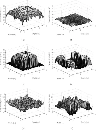
in section 2.1. The resultant received power distribution can be seen in Figure 2(a). As shown,
the received power has a range between 19.9µW and 56.7µW, a deviation of 36.8µW, or 65%
of the peak value. Furthermore, the bandwidth, as in Figure 2(c) varies between 14.6 MHz and
Important factors to note are the peaks and valleys within the received power distribution of
Figure 2(a). This is due to each receiver being aligned differently to ones at adjacent positions.
This variability, that is not only present from one environment to the next, but also from receiver
position within a given environment highlights the challenge which system designers face.
Upon optimisation of the transmitter ratios by application of the SUS based GA, the received
power distribution, shown in Figure 2(b), is reduced to a range varying between 10.7µW and
18.8µW, a deviation of 8.1µW, or 43% from the peak value. In comparison to the non-optimised
case, and defining the GA optimisation gain to be the improvement as a %, in the power
devia-tion between the non-optimised and optimised distribudevia-tions, the GA optimisadevia-tion gain for this
scenario is therefore 22%. Considering bandwidth, shown in figure 2(d), the GA has reduced
the peak bandwidth found within the room to 53.7 MHz, but the worst case, or guaranteed
minimum bandwidth, remains the same as in the non-optimised case at 14.6 MHz. The peak,
or worst case RMS delay spread, as shown in figure 2(f), has increased from 2.17 ns to 2.73 ns,
a reasonable compromise, given the reduced power deviation the GA has provided.
5.2 Optimisation Including User Movement
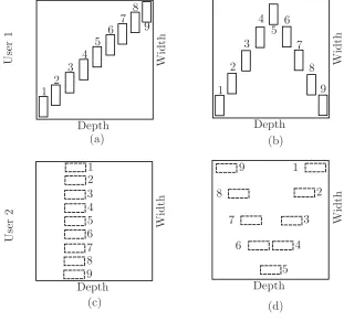
Within the established environment, two mobile users were subsequently incorporated. User 1
has a shoulder to shoulder width of 0.7 m, front to back depth of 0.4 m, and height of 1.8 m, and
is considered to have a reflectivity of ρ= 0.3. User 2 is identical, but with a reduced height of
1.6 m. User 1 and user 2 are simulated to have a movement pattern shown in figures 3 (a) and
occupy the same space at the same time.
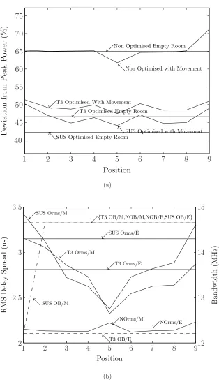
Figure 4(a) depicts the SUS based and tournament with 3 candidate (T3) selection scheme based
GAs for the optimised and non optimised power deviation at each movement position and when
empty. It shows the non optimised empty room power deviation is 65% (as per figure 2(a)),
which, upon user movement, is perturbed by up to 6%, with a range of 9% between 62% and
71%. After optimisation with the SUS based GA, the empty room deviation is reduced by 22% to
43% (as per figure 2(b)), with the maximum perturbation from user movement being increased
2% to 8%, whilst the range is reduced 3% to 6% as it varies between 44% and 50%. Application
of the T3 based GA, yields a reduction in power deviation of 18% to 47%, with the maximum
perturbation being reduced 2% to 4%, and the range is reduced 5% to 4% as it varies between
47% and 51%. Figure 4(b) depicts the associated optimised bandwidth (OB), non optimised
bandwidth (NOB), optimised RMS delay spread (Orms), and non-optimised RMS delay spread
(NOrms), when empty (/E), and with movement (/M), of the system. Here it is shown, similar
to the empty case, there is little penalty from applying the GA with < 2.5 MHz reduction in
bandwidth for the T3 scheme and<1.5 ns RMS delay spread penalty over the users’ movement
positions.
Finally, to provide further evidence of the ability of the GA to handle multiple dynamic
sce-narios, a second environment was created., This had the same dimensions as previously but the
ceiling, south and west walls had reflectivities increased toρ= 0.8, the east wall reflectivity was
reduced to ρ = 0.6 and the north wall reflectivity was reduced to ρ = 0.5. User 1 and User 2
were then modelled moving in a sequence of 9 positions, as depicted in Figures 3(b) and (d)
room power deviation is 73%, which, upon user movement, is perturbed by up to 8%, with a
range of 9% between 65% and 74%. After optimisation with the SUS based GA, the empty room
deviation is reduced by 27% to 46%, with the maximum perturbation being reduced 3% to 5%,
as the range is maintained at 9% as it varies between 42% and 51%. With the application of
the T3 based GA, the empty room deviation is reduced by 22% to 51%, with the maximum
per-turbation being reduced 1% to 7%, as the range is again maintained at 9% as it varies between
44% and 53%. Figure 5(b) provides the associated optimised bandwidth (OB), non-optimised
bandwidth (NOB), optimised RMS delay spread (Orms), and non-optimised RMS delay spread
(NOrms) when empty (/E), and with movement (/M) of the system. It can be seen that, similar
to the case of environment 1, the optimisation produces for the worst case <2.5 MHz reduction
in bandwidth and <1.5 ns RMS delay spread penalty over the users’ movement positions.
6
Conclusions
This paper has demonstrated further the novel approach of using a GA-controlled MSD
trans-mitter, capable of successfully optimising the received power distribution in multiple
environ-ments with multiple mobile users, each capable of randomly aligning their receivers. From the
evaluation of two tailored GAs, an optimisation gain of up to 27% can be achieved for empty
environments, whilst a gain of 26% can be achieved when the users are moving. Furthermore,
the user’s movement has been shown to be capable of perturbing the power distribution by up to
8%, which can be reduced to 5% upon application of this technique. The optimisation has also
been achieved with negligible bandwidth and RMS delay spread penalties, of < 2.5 MHz and
<1.5 ns respectively. Finally, this method has the potential to provide a highly adaptable
alignment and multiple user movement, in applications where cost and mobility are paramount.
References
[1] Green, R.J., Joshi, H., Higgins, M.D., and Leeson M.S.: ‘Recent developments in indoor
optical wireless systems.’, IET Commun., 2008, 2,(1), pp. 3–10.
[2] Hashemi, H., Yun, G., Kavehrad, M., Behbahani, F., and Galko, P.A.: ‘Indoor propagation
measurements at infrared frequencies for wireless local area networks applications.’ IEEE
Trans. Veh. Technol., 1994, 43, (3), pp. 562–576.
[3] Moreira, A.J.C., Valadas, R.T., and de Oliveira Duarte A.M.: ‘Optical interference
pro-duced by artificial light.’, Wireless Networks, 1997, 3, (2), pp. 131–140.
[4] Gfeller, F.R., and Bapst, U.: ‘Wireless in-house data communication via diffuse infrared
radiation.’, Proc IEEE., 1979, 67, (11), pp. 1474–1486.
[5] O’Brien, D.C., Katz, M., Wang, P., Kalliojarvi, K., Arnon, S., et al.: ‘Short Range Optical
Wireless Communications.’, Wireless World Research Forum., 2005.
[6] Djahani, P., and Kahn, J.M.: ‘Analysis of infrared wireless links employing multibeam
transmitters and imaging diversity receivers.’, IEEE Trans. Commun., 2000, 48, (12), pp.
2077–2088.
[7] Ramirez-Iniguez, R., and Green. R.J.: ‘Optical antenna design for indoor optical wireless
[8] Lee, D.C.M., Kahn, J.M., and Audeh, M.D.: ‘Trellis-coded pulse-position modulation
for indoor wireless infrared communications.’, IEEE Trans. Commun., 1997, 45, (9), pp.
1080–1087.
[9] Uno, H., Kumatani, K., Okuhata, H., Shirakawa, I., and Chiba, T.: ‘ASK digital
demod-ulation scheme for noise immune infrared data communication.’, Wireless Networks, 1997,
3, (2), pp. 121–129.
[10] Dickenson, R.J., and Ghassemlooy, Z.: ‘A feature extraction and pattern recognition
re-ceiver employing wavelet analysis and artificial intelligence for signal detection in diffuse
optical wireless communications.’, IEEE Trans. Wireless. Commun., 2003, 10, (2),pp. 64–72.
[11] Wong. D.W.K., Chen, G., and Yao, J.: ‘Optimization of spot pattern in indoor diffuse
optical wireless local area networks.’, Optics Express., 2005, 13, (8), pp.3000–3014.
[12] Wen, M., Yao, J., Wong, D.W.K., and Chen, G.C.K.: ‘Holographic diffuser design using a
modified genetic algorithm.’, Optical Eng., 2005, 44, (8), pp. 085801–8.
[13] Kirkpatrick, S., Gelatt, C.D., and Vecchi, M.P. ‘Optimization by Simulated Annealing.’,
Science., 1983, 220, (4598), pp. 671–680.
[14] Higgins, M.D., Green, R.J., and Leeson, M.S.: ‘A Genetic Algorithm Method for Optical
Wireless Channel Control.’, IEEE J. Lightwave. Tech., 2009, 27, (6), pp. 760–772.
[15] Higgins, M.D., Green, R.J., and Leeson, M.S.: ‘Genetic Algorithm Channel Control for
Indoor Optical Wireless Communications.’, Int. Conf. on Transparent Optical Networks
[16] Higgins, M.D., Green, R.J., and Leeson, M.S.: ‘Receiver alignment dependence of a GA
controlled optical wireless transmitter.’, J. of Optics A: Pure and Applied Optics., 2009,
11, (7), pp. 075403.
[17] Kahn, J.M., Krause, W.J., and Carruthers, J.B.: ‘Experimental characterization of
non-directed indoor infrared channels.’, IEEE Trans. Commun., 1995, 43, (234), pp. 1613–1623.
[18] Yang, H., and Lu, C.: ‘Infrared wireless LAN using multiple optical sources.’, IEE Proc.
Optoelectron., 2000, 147, (4), pp. 301–307.
[19] Jivkova, S., Hristov, B.A., and Kavehrad, M.: ‘Power-efficient multispot-diffuse
multiple-input-multiple-output approach to broad-band optical wireless communications.’, IEEE
Trans. Veh. Technol., 2004, 53, (3), pp. 882–889.
[20] O’Brien, D.C., Faulkner, G.E., Zyambo, E.B., Jim, K., Edwards, D.J., et al.: ‘Integrated
transceivers for optical wireless communications.’, IEEE J. Sel. Topics Quantum Electron.,
2005, 11, (1), pp. 173–183.
[21] Pohl, V., Jungnickel, V., and von Helmolt, C.: ‘Integrating-sphere diffuser for wireless
infrared communication.’, IEE Proc. Optoelectron., 2000. 147, (4), pp. 281–285.
[22] Komine, T., and Nakagawa, M.: ‘Fundamental analysis for visible-light communication
system using LED lights.’, IEEE Trans. Consum. Electron., 2004, 50, (1), pp. 100–107.
[23] Barry, J.R., Kahn, J.M., Krause, W.J., Lee, E.A., and Messerschmitt, D.G.: ‘Simulation
of multipath impulse response for indoor wireless optical channels.’, IEEE J. Sel. Areas.
[24] Carruthers, J.B., Carroll, S.M., and Kannan, P.: ‘Propagation modelling for indoor
op-tical wireless communications using fast multi-receiver channel estimation.’, IEE Proc.
Optoelectron., 2003, 150, (5), pp. 473–481.
[25] Carruthers, J.B, and Kannan, P.: ‘Iterative site-based modelling for wireless infrared
channels.’, IEEE Trans. Antennas. Propag., 2002, 50, (5), pp. 759–765.
[26] Carruthers, J.B., and Kahn, J.M.: ‘Modeling of nondirected wireless infrared channels.’,
IEEE Trans. Commun., 1997, 45, (10). pp. 1260–1268.
[27] Haratcherev, I., Taal, J., Langendoen, K., Lagendijk, R., and Sips, H.: ‘Automatic IEEE
802.11 rate control for streaming applications.’, Wireless Commun. Mob. Comput., 2005,
5, (4), pp. 421–437.
[28] Garcia-Zambrana, A., and Puerta-Notario, A.: ‘Novel approach for increasing the
peak-to-average optical power ratio in rate-adaptive optical wireless communication systems.’, IEE
Proc. Optoelectron., 2003, 150, (5), pp. 439–444.
[29] Pakravan, M.R., and Kavehrad, M.: ‘Indoor wireless infrared channel characterization by
measurements.’, IEEE Trans. Veh. Technol., 2001, 50, (4), pp. 1053–1073.
[30] B¨ack, T., Hammel, U., and Schwefel, H.P.: ‘Evolutionary Computation: Comments on the
History and Current State.’, IEEE Trans. Evol. Comput., 1997, 1, (1), pp. 3–17.
[31] Rothlauf, F.: ‘Representations for genetic and evolutionary algorithms.’, Springer, 2002.
[32] B¨ack, T.: ‘Evolutionary algorithms in theory and practice : evolution strategies,
evolution-ary programming, genetic algorithms.’, Oxford University Press, 1996.
[33] Baker, J.E.: ‘Reducing bias and inefficiency in the selection algorithm.’, Proc. 2nd Int.
[34] Poli, R.: ‘Tournament Selection, Iterated Coupon-Collection Problem, and
Backward-Chaining Evolutionary Algorithms.’, in Wright, A.H. (Ed.): ‘Foundations of Genetic
Rj,ElR Si,ElS
ˆ
n
{Si,ElS}
ˆ
n
{Rj,ElR}
φ
θ
FOVRj
R(φ)
D n= 50
n= 3
n= 1
A{Rj,ER
l }
r
{Rj,ElR}
r
[image:24.595.153.446.136.380.2]{Si,ElS}
Width (m) Depth (m) R ec ei ve d P ow er ( µ W ) 0 2 4 6 0 2 4 6 0 10 20 30 40 50 60 (a)
Width (m) Depth (m)
R ec ei ve d P ow er ( µ W ) 0 2 4 6 0 2 4 6 0 10 20 30 40 50 60 (b)
Width (m) Depth (m)
B an d wi d th (M Hz ) 0 2 4 6 0 2 4 6 0 10 20 30 40 50 60 70 (c)
Width (m) Depth (m)
B an d wi d th (M Hz ) 0 2 4 6 0 2 4 6 0 10 20 30 40 50 60 70 (d)
Width (m) Depth (m)
R M S D el ay S p re ad (n s) 0 2 4 6 0 2 4 6 0 0.5 1 1.5 2 2.5 3 (e)
Width (m) Depth (m)
[image:25.595.108.490.131.648.2]R M S D el ay S p re ad (n s) 0 2 4 6 0 2 4 6 0 0.5 1 1.5 2 2.5 3 (f)
Figure 2: Optimisation random receiver alignment using the SUS based GA. Power: (a)non
optimised, (b) optimised. Bandwidth: (c) non optimised, (d) optimised. RMS delay spread: (e)
1 1 1 1 2 2 2 2 3 3 3 3 4 4 4 4 5 5 5 5 6 6 6 6 7 7 7 7 8 8 8 8 9 9 9 9 Depth Depth Depth Depth W id th W id th W id th W id th U se r 1 U se r 2 (a) (b) (c) (d)
Figure 3: Movement positions of 2 users. (a) User 1, movement pattern 1. (b) User 1, movement
Position D ev ia ti on fr om P ea k P ow er (% )
ւNon Optimised Empty Room
տNon Optimised with Movement
տSUS Optimised with Movement
ւT3 Optimised Empty Room
ւT3 Optimised With Movement
տSUS Optimised Empty Room
1 2 3 4 5 6 7 8 9
40 45 50 55 60 65 70 75 (a) R M S D el ay S p re ad (n s) Position ւSUS Orms/M
տSUS OB/M
ւT3 Orms/M
ւ{T3 OB/M,NOB/M,NOB/E,SUS OB/E}
ւNOrms/M
ւNOrms/E ւSUS Orms/E
ւT3 Orms/E
տT3 OB/E
B an d wi d th (M Hz )
1 2 3 4 5 6 7 8 912
[image:27.595.143.457.122.669.2]13 14 15 2 2.5 3 3.5 (b)
Figure 4: Environment 1 multi user optimisation (a) Power deviation. (b) Bandwidth (- -) and
Position D ev ia ti on fr om P ea k P ow er (% )
ւNon Optimised Empty Room
տNon Optimised with Movement
տSUS Optimised with Movement
տT3 Optimised Empty Room
ւT3 Optimised with Movement
տSUS Optimised Empty Room
1 2 3 4 5 6 7 8 9
45 50 55 60 65 70 75 80 (a) R M S D el ay S p re ad (n s) Position տSUS Orms/M
ւ{SUS OB/M,T3 OB/M,NOB/M,NOB/E,SUS OB/E}
ւT3 Orms/M
ւNOrms/M ւNOrms/E
ւSUS Orms/E ւT3 Orms/E
տT3 OB/E
B an d wi d th (M Hz )
1 2 3 4 5 6 7 8 912
[image:28.595.144.454.129.668.2]13 14 15 16 2 2.5 3 3.5 4 (b)
Figure 5: Environment 2 multi user optimisation (a) Power deviation. (b) Bandwidth (- -) and
![Figure 1: Source, receiver and reflector geometry, adapted from [23].](https://thumb-us.123doks.com/thumbv2/123dok_us/9662246.468206/24.595.153.446.136.380/figure-source-receiver-reector-geometry-adapted.webp)