Munich Personal RePEc Archive
Qualitative variables and their reduction
possibility. Application to time series
models
Ciuiu, Daniel
Technical University of Civil Engineering Bucharest, Romanian
Institute for Economic Forecasting
June 2013
QUALITATIVE VARIABLES AND THEIR REDUCTION POSSIBILITY. APPLICATION TO TIME SERIES MODELS
DANIEL CIUIU1
1 Department of Mathematics and Computer Science, Technical University of Civil Engineering, Bucharest, Bd. Lacul Tei Nr.
124, Bucharest, Romania & Romanian Institute for Economic Forecasting, Str. 13 Septembrie 13, Bucharest, Romania, [email protected]
Abstract: In this paper we will study the influence of qualitative variables on the unit root tests for stationarity. For the linear regressions involved the implied assumption is that they are not influenced by such qualitative variables. For this reason, after we have introduced such variables, we check first if we can remove some of them from the model.
The considered qualitative variables are according the corresponding coefficient (the intercept, the coefficient of Xt−1and the coefficient of t), and on the different groups built tacking into account the characteristics of the
time moments.
Keywords: Qualitative variables, Dickey-Fuller, ARIMA, GDP, homogeneity.
1. INTRODUCTION
In the general case a time series can be decomposed in three parts [1, 3, 5]: the trend, the sesonal component and the stationary component. If there is no sesonnal component, a method to estimate and remove the trend is the moving average. The moving average of orderqis
b mt =
q
∑
j=−q Xt+j
2·q+1 . (1)
In [1] there are consideredXt=X1fort<1, andXt=Xnfort>n, and in [3] and [5] there are computed
only the values for whichq<t≤n−q, hence all the terms in the above relation exist in the time series. A criterion to chooseqused in [3] is the minimum variance ofXt−mbt.
If the above time seriesXt contains also a seasonal component, having the periods, then we remove first this
component as follows.
Consider two cases: s=2·q+1 ands=2·q. In the first case we estimatembt according(1), and in the
second case we estimate
b mt =
Xt−q+Xt+q
2 +
q−1
∑
j=−q+1
Xt+j
2·q . (2)
Next we compute the average yk of Xk+js−mbk+js for q<k+js ≤n−q, and from here the seasonal
component
b
ck=yk fork=1,s
b
ck=bck−sfork>s
. (3)
The time seriesXet=Xt−cbt has no more seasonal component, and we apply(1)(with anotherq) for removing
the trend. Obviously, the criterion to choosesandq1is the minimum variance of the obtained stationary time
series [3].
Another method to separate the three components is the differenciating method [1, 3, 5]. We denote first
∆Xt=Xt−Xt−1
∆sXt =Xt−Xt−s
wheresis the number of seasons.
The above operator∆is the difference operator, and the operator∆sis the seasonal difference operator, with
the periods. If the time seriesXt has a seasonal component with the periods, then there existsns>0 such that
Yt=∆nssXt (5)
has no seasonal component. Otherwise, considerYt=Xt. If the time seriesYt has trend, then there existsd>0
such that
Zt=∆dYt (6)
is stationary. Analogous to the case of lack of seasonal component, ifYt has no trend we haveZt =Yt.
◮Definition 1. The time seriesXt without seasonal component isARIMA(p,d,q)if the time seriesYt=∆dXt
isARMA(p,q).
The exponential smoothing is another method to obtain a stationary time series [1, 3, 5]. Starting from the initial time seriesXt and from the real numbera∈(0,1), we define
b m1=X1
b
mt =a·Xt+ (1−a)·mbt−1fort>1 . (7)
From here we obtain fort>1 by computations
b
mt = (1−a)t−1X1+
t−2
∑
j=0
a(1−a)jXt−j. (8)
We notice that the decrease of the coefficients ofXt,Xt−1,...,X2is exponential, and this justifies the name of
exponential smoothing.
The criterion for choosingais such that
t
∑
j=1
(Xt−mbt)2 (9)
is minimum [3].
To decide between time series models, we use unit root tests. One of them is the Dickey—Fuller test [3]. For this, consider the models
Xt =αXt−1+at, with |α|<1 (10a)
Xt =Xt−1+at (10b)
Xt =αXt−1+β+at, with |α|<1,β6=0 (10c) Xt =Xt−1+β+at, withβ6=0 (10d) Xt =αXt−1+β+γt+at,with |α|<1,γ6=0 (10e) Xt =Xt−1+β+γt+at, withγ6=0 (10f)
The above models(10b),(10d)and(10f)are stationary in differences, and the time series of these types are made stationary by differentiating. The models(10c)and(10e)are trend-stationary, and the time series according these models are made stationary by identification and removing trend (moving average, or exponential smoothing).
For the Dickey—Fuller test we group first into pairs the model(10a)with the model(10b), the model(10c)
∆Xt =ΦXt−1+at (11a)
∆Xt =ΦXt−1+β+at (11b)
∆Xt =ΦXt−1+β+γt+at (11c)
In fact the Dickey—Fuller test contains three sub-tests. We test first the signification of the coefficients for the linear regression model(11c), but forΦthe test must be left-sided:H0:Φ=0, andH1:Φ<0.
If after the first signification test it results thatΦis significant, it results that the right model from(10)is
(10e)ifγis significant (the autoregressive model with temporal trend),(10c)ifγis not significant, butβis significant (the autoregressive model with drift), and, if the other two parameters are not significant, we accept the model(10a)(the autoregressive model).
If in the first testΦis not significant, we proceed to test the signification of the coefficients of the regression model(11b). IfΦbecomes significant, then we choose between the models(10c)and(10a), depending on the signification ofβ. Otherwise, we do the last test, namely the test for signification ofΦin the model(11a).
If in the last testΦis significant, we accept the model(10a). Otherwise (ifΦis not significant in all the three tests), we accept the model(10f)ifγwas significant in the first test (random walk with drift and trend),
(10d)ifγwas not significant in the first test, butβwas significant in the second test (random walk with drift), respectively(10b)ifγwas not significant in the first test, andβwas not significant in the second test (random walk).
We cannot use the Student test for the signification ofΦ,βorγ. This, because ifΦ=0 orγ6=0Xt is not
stationary, for any values ofβ, hence the common rules of statistical inference (particulary, the Student test) cannot be applied [3]. Dickey and Fuller have estimated by the Monte Carlo method the critical values (instead of the quantiles of Student distribution) with which we have to compare the computed Student statistics forΦ, in the cases of different sizes of time series.
For the qualitative explanatory variables, in [3] there is presented the problem of the dependence of income in terms of number of school years, formgroups. There are obtained the two linear regressions
Y =a(0j)+a1X, (12)
wherea(0j)is the intercept for the group j. Considering the dummy variables
Dj=
1 for the groupj+1
0 otherwise , j=1,m−1 (13)
it is obtained the linear regression
Y =a(01)+
m−1
∑
j=1
a(0j+1)−a(0j)
Dj+a1X. (14)
In the same manner there are considered the seasonal data. In this case the number of groups is the number of seasons.
In the above cases the slope is common, and the intercept differs from a group to another. If the slope differs, we denote byDj,0the above dummy variables, and the other qualitative explanatory variables are
Dj,1=
Xfor the groupj+1
0 otherwise , j=1,m−1. (15)
Finally we obtain the linear regression
Y =a(01)+
m−1
∑
j=1
a0(j+1)−a0(j)Dj,0+a( 1) 1 X+
m−1
∑
j=1
a1(j+1)−a1(j)Dj,1. (16)
1. A preasure on nominal revenues, either in the private or in the budgetary sector, remains significant. The index of expected disposable income ranges between 1.06 and 1.085.
2. After the elaboration of the 2005 version of the elaboration of the 2005 version of the macromodel, some factors infered and negatively influenced the global return of the Romanian economy. This impact was accentueted during the crisis. Therefore the equation for the total factor productivity, and for the unemployment rate were corrected for all the years of the economic crises. In the case of gross fixed capital formation the correction was for the first two years of the period.
3. The international financial crisis will pass into a moderate global recovery. The parameters concerning the world trade index in real terms and world trade deflator are considered as slowly ascending series, and the short term interest rate is constant.
4. It is expected that the capital flows will increase. This comes from portofolio investments or the net tranfers from abroad, and from a rising degree of absorption of the European structural and cohesion funds.
5. The general consolidated budget is conceived under stability of taxation. Therefore the ratio of direct taxes to GDP, the ratio of other budget revenues to GDP and the ratio of VAT to gross value added are constant.
6. The annual index of broad money (IM2) is projected to exceed slightly the similar index of expected disposable income (IYd), which allows a reduction in interest rates.
7. The rate of tangible fixed assets depreciation is mentained at constant level of 0.075.
For the second scenario (the worsened scenario W1Sc), which generally mentains the assumptions of base scenario, it assumes that the domestic situation (institutional reforms, fiscal systems, etc.) does not allow a significant improvement of the business environment. Consequently, in addition to the base scenario there are considered the following assumptions:
1. The capital inflows are more limited, and this concerns the foreign direct and portofolio investments, current account net transfers and structural European funds.
2. The relationship for total factor productivity is also penalized by slightly increase negative correction coefficients.
3. NBR policy remains able to mentain the exchange rate of RON in a narrow band of fluctuation.
The third scenario (the worsened scenario W2Sc) is derived from the previous one, but it tries to compress the inflation by more restrictive income, monetary and budget expenditure policies. The additional assumptions are as follows:
1. A slower increase in expected disposable income is taken into account.
2. The exogeneous coefficients regarding government transfers and other public expenditures are also reduced in comparison with the other two scenarios.
3. The broad money supply is projected at lower levels.
2. THE TEST FOR IDENTITY OF COEFFICIENTS OF QUALITATIVE VARIABLES
In this section we consider not only one set of coefficientsΦ, βandγin (11): we havegrgroups and we consider a set of above mentioned coefficients for each group.
A test for identity of some expectation is the Tukey test [2]. Considermindependent samples having the distributionsN µi,σ2
, having the same size,n.
The Tukey test checks with the first degree errorεthe null hypothesisH0:µ1=µ2=...=µm against the
alternative hypothesisH1: there existi6= jsuch thatµi6=µj.
Consider an unbiased estimator ofσ2based upponrdegrees of freedom, and we denote it byS2. We compute
the statistics
q=Xmax−Xmin
S· q
2
n
, (17)
whereXmaxandXminare the maximum, respectively minimum expectation of the abovemsamples.
It is proved [2] that theqhas the Student distribution withrdegrees of freedom. Therefore we accept the null hypothesis if and only ifq<tr;ε2, wheretr;ε2 is the quantile of the error 2ε of the Student distribution withr
◮Remark ([2]). The denominator from(17),S·
q 2
n, is in fact the estimator of the standard deviation of the
numerator,Xmax−Xmin, withrdegrees of freedom. Therefore the Tukey test can be performed also in the case
of different variancesσ2
i. It is enough to consider the same degrees of freedom,r, and the statistics becomes q= max
i,j=1,m
|Xi−Xj| √
S2
i+S2j
, whereXiandS2i are the estimators of the expectation and of the variance of the componenti,
the last one being computed withrdegrees of freedom.
If we want to check if some regression coefficients are equal, with given first degree errorε, we consider the formula for the variance-covariance matrix of the vector of coefficients,Ab[3]:
VarAb=σ2u(X′X)−
1
, (18)
where σ2
u is the estimator of the variance of errors. The number of degrees of freedom (for residues and
coefficients) isn−k−1, wherenis the size of data andkis the number of explanatory variables. Therefore the Tukeyq−statistics becomes
q= max
i,j=1,m
Xi−Xj
q
S2
i +S2j−2·Ci,j
, (19)
whereXi andS2i are the estimators of the expectation and of the variance of the coefficientAi, andCi,j is the
covariance of the coefficientsAiandAj. Of course, the above maximum range only for the pairs(i,j)such that,
according to null hypothesis, we haveAi=Aj, and the number of degrees of freedom is alson−k−1.
Therefore for common regression coefficients we compare the aboveq−statistics with the quantiletn−k−1;ε2.
We accept the null hypothesis of identical coefficients if and only ifq<tn−k−1;2ε. This test can be performed not
only to check if one group of coefficients has a single value. We can check for instance if the coefficients ofX1
andX2are identical, and in the same time the coefficients ofX3andX4are identical, but the coefficients ofX1
andX3are not necessary identical.
The regression coefficients can be considered also for qualitative/ dummy explanatory variables. The conditions that have to be fulfilled are the mutual independence ofYtand ofXit. Therefore in the time series case
we cannot use the Student distribution for testing the identity of coefficients, for the same reasons we cannot use it for unit root tests.
More exactly, consider the equation(11). The set of parameters(Φ,β,γ)is replaced bygrsets(Φi,βi,γi)i=1,gr
corresponding togrgroups. The qualitative variables are
XtD−i1;i
ti
=
Xt1−1
t
(20)
for the groupi, and the corresponding set of coefficients is
Φβii
γi
.
Thegrgroups are built taking into account the time period (the moment belongs to the economic crisis or not, or, for trimestrial or monthly data, to a given trimester or month).
For each test from the Dikey—Fuller methodology mentioned in introduction, each involved signification test is preceded by homogeneity tests as follows:
1. First we test the total homogeneity: the involved parameter has the same value for all groups.
2. If the total homogeneity fails, we remove a component using the minmax criterion: if we remove a component, the corresponding statistics for identity of the retained coefficients is minimum.
3. If for a partial homogeneity test we accept the null hypothesis, we stop, considering the retained coefficients having the same value. Otherwise, we continue with the above minmax technique, until it remains only one coefficient, or we accept the identity for some coefficients.
the interval is(−1,0). If the alternative is6=0 (as forγandβ), the interval is(−1,1). We generate also the variance ofet in the interval(0,1). Of course, for identity between some parameters we do not generate all the
coefficients: we generate only one coefficient for each group of equal coefficients. For each set of parameters we generate 10000 such models.
We compute for each model the q−statistics, we order the 10000000q−statistics. Because we use also the absolute value, the quantile is the value from the position 10000000(1−ε)instead those from the position 10000000 1−ε2.
The parameters for each of the above models are generated uniform on the interval(−1,1) forβandγ coefficients, on the interval(−1,0)forΦcoefficients, respectively on the interval(0,1)for the variance of the
errors. The errors are generated as normal variables wis the expectation zero and the variance generated before. The methods to generate the above random variables, and methods to solve optimization problems are presented in [6]. From the methods to generate normal variables presented in the above book, we choose the Box—Muler method, because it is the most rapid.
For signification we use the standard Dickey—Fuller test if after the homogeneity test we conclude that we have only one group for all coefficients. Otherwise we estimate the quantiles by simulation, and we use two-sided tests. Even forΦ, due to the existence of several groups, we can have positive values.
3. APPLICATION
Consider the yearly data of GDP in the period 1990-2011. The data are from [7]. The three periods are 1990-2000, 2001-2007 and 2008-2011 (the economic crisis) inclusive.
In the case of pure data we obtain first, using ourC+ +program, the regression
∆Xt = 20.79444D1−108.38084D2−269.04604D3−0.84321Xet−1;1−0.22976Xet−1;2−0.55302Xet−1;3+
1.28323et1+10.08695et2+17.93309et3.
The variance of the residues isσ2
u=24.05647, and theq−statistics using the mentioned minmax technique
are 2.51044 (obtained for the first two periods, years 1990—2008) and 1.02822 (obtained for the last two periods, years 2001—2011) forγ, 1.59709 (obtained for the first two periods) and 0.62695 (obtained for the
first and the last period, years 1990—2001 and 2008—2011) forΦ, respectively 3.23053 (obtained for the first two periods) and 0.85615 (obtained for the the last two periods) forβ.
We order the above q-statistics, and we obtain the following sequence of tests:
1. Φi=Φ,γi=γandβi=β.
2. Φi=Φ,γi=γandβ2=β3.
3. Φi=Φ,γ2=γ3andβ2=β3.
4. γ2=γ3,β2=β3andΦ1=Φ3.
5. Possible differentγi,β2=β3andΦ1=Φ3.
6. Possible differentγiandβi, andΦ1=Φ3.
Comparing to the quantiles from Table 1, we accept the null hypothesis in the case of the first test, with the threshold of 5%1. Therefore we do not proceed to do the other five tests.
Table 1: The quantiles for the homogeneity tests in the case of first degree error being 10%, 5%, 2.5%,
respectively 1%.
Model Test Quantiles
10% 5% 2.5% 1% III Φi=Φ,βi=βandγi=γ 3.25943 3.82568 4.39094 5.17224
II βi=βandΦi=Φ 2.35455 2.71764 3.06432 3.49962
II βi=βandΦ1=Φ2 2.35467 2.72891 3.08986 3.55251 II β1=β2andΦ1=Φ2 2.02454 2.40515 2.76983 3.22623 I Φi=Φ 1.93702 2.27258 2.58109 2.97614
I Φ1=Φ3 1.49849 1.83887 2.1422 2.53485
For the equation(11b)we obtain the regression
∆Xt =13.85923D1+3.43493D2+209.915D3−0.40747Xet−1;1+0.22203Xet−1;2−1.24332Xet−1;3.
The variance of residues isσ2
u=52.55795, and the lists of q-statistics is 6.15478 (obtained for the last two
periods) and 1.43677 (obtained for the first two periods) forΦ, respectively 5.07655 (obtained for the last two
periods) and 0.65238 (obtained for the first two periods) forβ.
We order the above q-statistics, and we obtain the following sequence of tests:
1. βi=βandΦi=Φ.
2. βi=βandΦ1=Φ2.
3. Φ1=Φ2andβ1=β2.
4. Possible differentΦi, andβ1=β2.
In the case of the first test we reject the null hypothesis for 5%, because 6.15478>2.71764. The same thing we can say about the second test, because 5.07655>2.72891. We notice that the above statistics are also significant for 1%.
In the case of the third test, we accept the null hypothesis for 5%, because 1.43677<2.40515. The statistics is significant neither for 10%.
For the equation(11a)we obtain the regression
∆Xt=−0.004Xet−1;1+0.25366Xet−1;2−0.05185Xet−1;3.
The variance of residues isσ2
u=126.32111, and the list of q-statistics is 5.34024 (obtained for the last two
periods) and 0.44964 (obtained for the first and the last period).
We test first if all the values ofΦiare identical, and we reject the null hypothesis for 5%, because 5.34024>
2.27258, and the statistics is also significant for 1%.
Next we test first ifΦ1=Φ3, and we accept the null hypothesis for 5%, because 0.44964<1.83887. The
statistics is neither significant for 10%.
In the case of logarithmic data, we obtain first the regression
∆Xt = 2.55954D1+1.07965D2+0.59702D3−0.79454Xet−1;1−1.34646Xet−1;2−0.53005Xet−1;3+
0.03795et1+0.33396et2+0.105et3.
The variance of the residues isσ2
u=0.00582, and the list ofq−statistics is 1.6956 (obtained for the first two
periods) and 0.6333 (obtained for the first and the last period) forγ, 0.74806 (obtained for the first two periods)
and 0.30465 (obtained for the first and the last period) forΦ, respectively 1.82297 (obtained for the first two periods) and 0.07644 (obtained for the last two periods) forβ.
We order the above q-statistics, and we obtain the following sequence of tests:
1. Φi=Φ,γi=γandβi=β.
2. Φi=Φ,γi=γandβ2=β3.
3. Φi=Φ,γ1=γ3andβ2=β3.
4. γ1=γ3,Φ1=Φ3andβ2=β3.
5. Possible differentγi,Φ1=Φ3andβ2=β3.
6. Possible differentγiandΦi, andβ2=β3.
Because the statistics 1.82297 is less than the same quantile of 5% from the case of pure data, we accept also the null hypothesis of total homogeneity. We accept also the null hypothesis for the threshold of 10%, as for pure data.
For the equation(11b)we obtain the regression
∆Xt=1.30746D1+0.13816D2+6.445D3−0.37205Xet−1;1+0.02095Xet−1;2−1.25707Xet−1;3.
The variance of residues isσ2
u=0.01384, and the lists of q-statistics is 1.88925 (obtained for the last two
periods) and 1.25023 (obtained for the first and the third period) forΦ, respectively 1.81271 (obtained for the last two periods) and 1.30958 (obtained for the first two periods) forβ.
1. βi=βandΦi=Φ.
2. βi=βandΦ1=Φ3.
3. β1=β2andΦ1=Φ3.
4. Possible differentβi, andΦ1=Φ3.
For the first test we accept the null hypothesis for 5%, and the statistics of 1.88925 is neither significant for
10%.
For the equation(11a)we obtain the regression
∆Xt=0.00051Xet−1;1+0.0523Xet−1;2−0.00739Xet−1;3.
The variance of residues isσ2
u=0.01636, and the list of q-statistics is 3.32351 (obtained for the first two
periods) and 0.43747 (obtained for the first and the last period).
For this model we perform the same test and we have the same conclusions and significance levels as in the case of pure data.
In the following we will test the signification of coefficients considering the resulting homogeneity. In the case of pure data, we test first the signification of the model
∆Xt=β+ΦXt−1+γt.
We obtain
∆Xt=−6.20162−0.20553Xt−1+2.51461t,
and the variance of residues is 246.8959. The Dickey—Fuller statistics are−0.085175 forβ,−1.73753 forΦ, and 2.34101 forγ.
In this case we perform the standard Dickey—Fuller test, model(11c). It results thatΦis not significant for 5%, because−1.73753>−3.6 forn=25, and the threshold decrease withn. The same thing we can say about the threshold for 10% andn=25,−3.24.
Next we test the signification of parameters for the model
∆Xt=β1,2D1,2+β3D3+Φ1,2Xet−1;1,2+Φ3Xet−1;3.
We obtain
∆Xt =−7.99486D1,2+209.915D3+0.31148Xet−1;1,2−1.24332Xet−1;3,
and the variance of residues is 69.76394. The statistics are−2.31095 forβ1,2, 4.53263 forβ3, 5.96962 forΦ1,2,
and−2.86293 forΦ3.
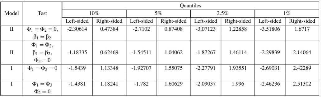
For the right-sided signification of Φ1,2 we have to compare the statistics 5.96962 with the 5% quantile,
which is 0.87408. It results thatΦ1,2is right-significant, hence the model is exploding for the period before
crisis. The statistics is significant also for 1%, when the quantile is 1.6717. ForΦ3, we compare the statistics of −2.86293 with the 5% threshold,−1.54511. The statistics is also significant for 1%. Therefore the series is
exploding before crisis, and stationary during it.
The above quantiles are listed in Table 2. We do not need now to check the significance ofβcoefficients, but we can conclude, using the two-sided thresholds from Table 3, thatβ1,2is significant for 10%, but it is not for at
Table 2: The quantiles for the one-sided signification tests forΦin the case of first degree error being 10%, 5%,
2.5%, respectively 1%.
Quantiles
Model Test 10% 5% 2.5% 1%
Left-sided Right-sided Left-sided Right-sided Left-sided Right-sided Left-sided Right-sided II Φ1=Φ2=0, -2.30614 0.47384 -2.7102 0.87408 -3.07123 1.22858 -3.51806 1.6717
β1=β2 Φ1=Φ2,
II β1=β2, -1.18335 0.62469 -1.54511 1.04062 -1.87267 1.46114 -2.29839 2.14064 Φ3=0
I Φ1=Φ3=0 -1.5439 1.13348 -1.92707 1.55075 -2.27791 1.93551 -2.69031 2.42289
I Φ1=Φ3 -1.4381 1.18241 -1.782 1.60629 -2.09037 1.996 -2.46236 2.51302 Φ2=0
Table 3: The quantiles for the two-sided signification tests forβin the case of first degree error being 10%, 5%,
2.5%, respectively 1%, Model II.
Test Quantiles
10% 5% 2.5% 1% β1=β2=0,Φ1=Φ2 2.02645 2.40952 2.76976 3.21575 β1=β2,Φ1=Φ2,β3=0 1.83231 2.20667 2.54475 2.9877
Finally, we test the signification of parameters for the model
∆Xt=Φ1,3Xet−1;1,3+Φ2Xet−1;2.
We obtain
∆Xt =−0.04605Xet−1;1,3+0.25366Xet−1;2,
and the variance of residues is 119.69177. The statistics are−1.36267 forΦ1,3, and 5.97619 forΦ2.
Comparing to the 5% thresholds, we conclude thatΦ1,3is not significant, even for 10%, andΦ2is significant
even for 1%. Therefore the GDP series is random walk for the periods 1990—2001 and 2008—2011, and exploding during the economic increasing period, 2001—2008.
In the case of logarithmic data, we test first the signification of the model
∆Xt=β+ΦXt−1+γt.
We obtain
∆Xt =0.82185−0.29444Xt−1+0.03963t,
and the variance of residues is 0.01863. The Dickey—Fuller statistics are 2.60596 forβ,−2.76856 forΦ, and
3.34774 forγ. We have again−2.76856>−3.24, henceΦis significant neither for 10%. Next we test the signification of parameters for the model
∆Xt=β+ΦXt−1.
We obtain
∆Xt =−0.04464+0.02941Xt−1,
and the variance of residues is 0.02864. The statistics are−0.19983 forβ, and 0.53683 forΦ.
BecauseΦ>0, it results that it is not significant from the Dickey—Fuller test point of view.
∆Xt=Φ1,3Xet−1;1,3+Φ2Xet−1;2.
We obtain
∆Xt =−0.00242Xet−1;1,3+0.0523Xet−1;2,
and the variance of residues is 0.01565. The statistics are−0.28404 forΦ1,3, and 4.84361 forΦ2.
Comparing to the 5% thresholds, we rich to the same conclusions as in the case of the pure data.
4. CONCLUSIONS
In this paper we have study the way we can group data only from the point of view of stationarizing time series. Two groups that have identical coefficients can be stationarized together, using the same scheme. An open problem is to extend the study for stationary data. More exactly, to test if two groups have the same AR and/ or MA coefficients, and/ or the same variance of white noise.
After we will make the groups after the homogeneity tests, considering also the ARMA structure and the variances of the white noises, we can build the scenarios of forecast depending on the group such that the future valueXn+1belongs to.
We notice that the logarithmic data are more homogeneous than the pure data. The explanation could be that the differences between values decrease if we apply logarithms. Moreover, for instance an exploding time serries becomes random walk by logarithm.
For only one sequential criterion to group the time moments we have made copies for the common years 2001 and 2008. The same thing we can do for several sequential criteria: we make only one sequential criterion, considering all the separation years from the considered criteria.
An open problem is to study the homogeneity for one or more seasonal criteria. If it is one criterion, we change the signification of groups. For instance, if we consider trimestrial data, T1 has the following new signification: Xt is inT1, andXt−1is inT4, and so on. If we have several periodic criteria, we make only one,
with one period equal to the highest common factor of the periods.
More difficult is the case when we have several criteria sequential and periodical. Of course, as we have mentioned above, we can reduce the problem to the case of two criteria: one sequential, and one periodical. This reduced case is also an open problem.
For the standard significance level of 5% we notice that in the case of the model(11b)we accept identical coefficients for the two periods before the economic crisis. Therfore the economic crisis is separated. In the case of the model(11a)we have another separation: we accept identicalΦcoefficients for the first and last periods, and the separated period is those from the middle (2001—2008), of the economic increase.
The identity of coefficients for two periods (first two in the case of model II, first and third in the case of model I) does not mean that we have the same time series. It means that we can use the same stationarising method (differences). The obtained stationary time series can be different.
REFERENCES
[1] Brockwell, P.J. & Davis, R.A. (2002). Springer Texts in Statistics; Introduction to Time Series and Forecasting. Springer-Verlag.
[2] Ciucu, G. & Craiu, V. (1974). Inferen¸t˘a statistic˘a. Bucharest: Ed. Didactic˘a ¸si Pedagogic˘a (English:
Statistical Inference).
[3] Jula, D. (2003). Introducere în econometrie. Bucharest: Professional Consulting (English: Introduction to
Econometrics).
[4] Dobrescu, E. (2010). Macromodel Simulations for the Romanian Economy. Romanian Journal of Economic Forecasting, XIII(2), 7-28.
[5] Popescu, Th. (2000). Serii de timp; Aplica¸tii la analiza sistemelor. Bucharest: Editura Tehnic˘a (English:
Time Series; Aplications to Systems’ Analysys).
[6] V˘aduva, I. (2004). Modele de simulare. Bucharest University Printing House.