Munich Personal RePEc Archive
Trend shocks and the countercyclical
U.S. current account
Amdur, David and Ersal Kiziler, Eylem
Muhlenberg College, University of Wisconsin-Whitewater
January 2012
Online at
https://mpra.ub.uni-muenchen.de/40147/
Trend Shocks and the Countercyclical U.S. Current Account
∗David Amdur Muhlenberg College†
Eylem Ersal Kiziler
University of Wisconsin-Whitewater‡
This Version: January 2012
Abstract
From 1960–2009, the U.S. current account balance has tended to decline during expansions and improve in recessions. We argue that trend shocks to productivity can help explain the countercyclical U.S. current account. Our framework is a two-country, two-good real business cycle (RBC) model in which cross-border asset trade is limited to an international bond. We identify trend and transitory shocks to U.S. productivity using generalized method of moments (GMM) estimation. The specification that best matches the data assigns a large role to trend shocks. The estimated model generates a countercyclical current account without excessive consumption volatility.
JEL Classification: E21, E32, F32, F41
Keywords: Current account, trend shocks, business cycles, open economy macroeconomics, DSGE models, GMM estimation
∗The authors would like to thank Ha Nguyen, Yamin Ahmad, and two anonymous referees for helpful comments. We also received many useful comments on earlier versions of this work from Martin Evans, Dale Henderson, Pedro Gete, Rudolfs Bems, and seminar participants at the Georgetown Center for Economics Research and the Midwest Economics Association. David gratefully acknowledges research funding from Muhlenberg College. Any mistakes are our own.
†Corresponding author. Department of Accounting, Business and Economics, 2400 Chew Street, Allentown, PA 18104, USA. Tel: 484-664-3257. E-Mail: [email protected].
1
Introduction
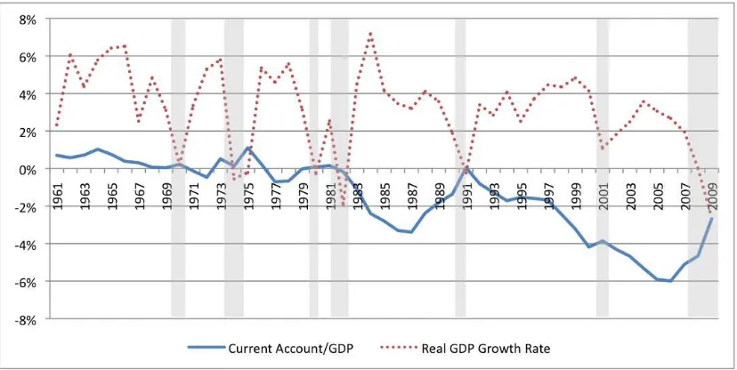
From 1960–2009, the U.S. current account balance has been countercyclical: the U.S. borrows more
from foreigners when output is growing rapidly, and less in recessions (Figure 1). Recent experience
provides a striking illustration. During the expansion of 2001–2006, the U.S. current account deficit
grew from 4% to 6% of GDP, prompting widespread concern about “global imbalances.” In the
aftermath of the financial crisis and subsequent recession, there was a dramatic correction, with
the deficit retreating to about 2.7% of GDP in 2009. The graph suggests a broad pattern of
current account decline during business cycle expansions and improvement just before and during
recessions. This pattern appears particularly striking after 1980.
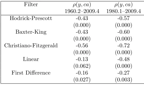
Table 1 offers quantitative evidence that the U.S. current account is countercyclical. We
ob-tained quarterly data on log U.S. real GDP and the current-account-to-GDP ratio and filtered
it in three different ways: with a Hodrick-Prescott filter, a Baxter-King band-pass filter, and a
Christiano-Fitzgerald random walk filter.1 We also analyzed deviations from a linear trend and
first differences. Over the time span 1960–2009, the correlation coefficient is negative in all five
specifications, and it is significantly different from zero in all except the linear trend. As suggested
by Figure 1, the pattern is even stronger over the time period 1980–2009. The negative
correla-tion coefficient over this time span is significantly different from zero in all five specificacorrela-tions. We
conclude that the U.S. current account is countercyclical.
Countercyclical current account balances are often associated with emerging economies. Aguiar
and Gopinath (2007) document that, on average, external balances are more strongly
countercycli-cal in emerging countries than in small open developed economies. They successfully reproduce
this pattern in a small open economy model with stochastic shocks to the trend growth rate of
pro-ductivity. The key insight comes from the permanent income hypothesis: a positive shock to trend
growth raises permanent income by more than current income. Domestic households respond
op-timally by borrowing against higher expected future income, opening up a current account deficit.
In contrast, a positive transitory shock raises current income by more than permanent income,
prompting households to save. Depending on the strength of the investment response, a transitory
1
Figure 1: U.S. current account balance as a share of GDP, and U.S. real GDP growth rate. Shaded bars are NBER recessions. Source: BEA.
shock causes either a smaller current account deficit or a current account surplus. The story is
then that emerging economies face relatively more volatile trend shocks than developed countries
do, which makes their trade and current account balances more countercyclical.
We argue that trend shocks are more important for the U.S. than received wisdom might suggest.
Our framework is a two-country DSGE model with perfectly observable trend and transitory shocks
to productivity. We estimate the model using quarterly data from 1960–2009. The specification
that best matches the data assigns a large role to trend shocks. The estimated model successfully
generates a countercyclical (traditional) current account balance.2 Moreover, the model does so
without generating excessive consumption volatility – a feature of emerging markets that is not
shared by the U.S. We conclude that trend shocks to productivity are a plausible driver of the
countercyclical U.S. current account.
Our findings do not preclude a role for investment in explaining U.S. current account dynamics.
Clearly U.S. investment increases in booms and falls in recessions. Holding national saving constant,
the investment response alone would make the current account countercyclical. However, national
saving is not constant over the business cycle. In particular, private consumption is procyclical.
2
Filter ρ(y, ca) ρ(y, ca) 1960.2–2009.4 1980.1–2009.4
Hodrick-Prescott -0.43 -0.57
(0.000) (0.000)
Baxter-King -0.43 -0.60
(0.000) (0.000) Christiano-Fitzgerald -0.56 -0.72
(0.000) (0.000)
Linear -0.13 -0.48
(0.062) (0.000)
First Difference -0.16 -0.27
[image:5.612.180.430.82.231.2](0.027) (0.003)
Table 1: Business cycle correlations between log U.S. real GDP (y) and the current-account-to-GDP ratio (ca). Data is quarterly. We set the smoothing parameter of the Hodrick-Prescott filter to 1600. The Baxter-King and Christiano-Fitzgerald filters were set to preserve components of the data with period between 6 and 32 quarters. After applying each filter, the resulting “business cycle” time series were demeaned, if the mean was significantly different from zero. Values in parentheses are significance levels of the correlation coefficient. Data is from the BEA.
We analyze the joint dynamics of consumption and investment in response to different shocks and
use these dynamics to predict the cyclicality of the current account.
There is a very large literature on the topic of whether U.S. GDP has a unit root; see, for
example, Lumsdaine and Papell (1997) and references therein. Our read of this literature is that it
is inconclusive. Indeed, the difficulty of detecting a unit root in a finite time series is a well-known
empirical issue. Christiano and Eichenbaum (1990) famously argued that postwar U.S. data does
not provide a long enough time span to plausibly determine whether U.S. GNP has a nonstationary
component. Instead, following Aguiar and Gopinath (2007), we take a structural approach and
analyze the effects of trend and transitory productivity shocks on agents’ optimizing behavior and
implied business cycle moments, with special attention to the correlation of the current account
with output. A similar structural approach is taken by Cochrane (1988), Campbell and Deaton
(1989), and Blundell and Preston (1998).
Our paper differs from Aguiar and Gopinath (2007) in that we use a two-country model, rather
than a small open economy. A two-country model is the convention in the literature when studying
international business cycles from the U.S. perspective (see, e.g., Backus et al. (1992), Baxter
and Crucini (1995), and Heathcote and Perri (2002)). Whereas a small country like Mexico can
valid for the U.S. Indeed, Aguiar and Gopinath (2007) do not analyze the U.S. To our knowledge,
our paper is the first to apply the methodology of Aguiar and Gopinath (2007) to study the business
cycle properties of the U.S. current account in a two-country framework.
Recent work has highlighted the effect of long-lived supply shocks on U.S. current account
dynamics. Much of this literature focuses on low frequency evolution. Engel and Rogers (2006),
building on Obstfeld and Rogoff (2005), develop a perfect foresight model cast in terms of country
shares of world output. They conclude that expectations of a rising share of U.S. in world output
can explain the large U.S. current account deficit. Also in a perfect foresight setting, Chen et al.
(2009) show that a gradual rise in the relative U.S. total factor productivity (TFP) growth rate
can explain the secular decline in the U.S. current account balance. Our findings support the
conclusions of these papers by offering new evidence that trend shocks to productivity are large
for the U.S. We also complement previous work by emphasizing the implications of trend shocks
at business cycle frequencies. We focus on explaining the countercyclical nature of the current
account: why the U.S. borrows more in booms and less in recessions.
Another strand of the literature focuses on disentangling the effects of trend and transitory
shocks for the U.S. Working with an empirical present-value model of the current account, Corsetti
and Konstantinou (2011) identify trend and transitory shocks by imposing a set of cointegrating
relationships on net output, consumption, and gross foreign assets and liabilities (at market value).
They find that consumption is largely driven by permanent shocks. Hoffmann et al. (2011) employ
a DSGE framework in which agents have imperfect information about the trend and transitory
shocks hitting the economy. They conclude that agents’ expectations about future TFP growth can
explain both the secular decline in the current account from 1995–2006, as well as the correction that
followed. We take a different but complementary approach. Following Aguiar and Gopinath (2007),
we assume perfect information and estimate the parameters governing the trend and transitory
shock processes using GMM estimation.
Nguyen (2011) also estimates volatilities of trend and transitory productivity shocks for the
U.S., focusing on the comovement of the (traditional) current account with valuation effects. We
focus instead on the comovement of the (traditional) current account with output, abstracting
whereas Nguyen (2011) looks at low-frequency evolution.3
Some recent papers have been critical of the Aguiar and Gopinath (2007) finding that “the cycle
is the trend” for emerging countries. Garcia-Cicco et al. (2010) estimate a small open economy
RBC model using Argentine and Mexican data over a much longer time span and find that the
model fits the data poorly over the long sample. Despite this finding, we believe that an RBC
framework can shed light on the relative importance of trend versus transitory productivity shocks
in the U.S. Our time span is considerably longer than in Aguiar and Gopinath (2007) and contains
about seven business cycles, versus the one-and-a-half to two business cycles in the time span
critiqued by Garcia-Cicco et al. (2010). Furthermore, our use of a two-country model allows foreign
productivity shocks to impact macro variables in the home country, allowing for a somewhat richer
set of disturbances than simply trend and transitory productivity shocks at home.4
The rest of the paper proceeds as follows. Section 2 describes the model. Section 3 documents
the baseline calibration and develops intuition with impulse response functions. Section 4 presents
our estimates of the parameters governing the trend and transitory shock processes and compares
simulated business cycle moments with the data. Section 5 concludes.
2
Model
The model is a two-country, two-good DSGE model with trend and transitory productivity shocks.
We assume that households can perfectly identify trend from transitory shocks. Markets are
incom-plete, because the only financial asset traded internationally is a non-contingent bond. We index
country-specific variables with the superscript i∈ {H, F}, where H is the home country and F is
foreign.
3
Relative to Nguyen (2011), the structure of goods and asset markets is also different: our model has two goods and one bond, whereas Nguyen (2011) has one good and two equities.
4
2.1 The production function
Each country is populated with a unit mass of identical, perfectly competitive firms that produce
a country-specific, traded good using capital and labor:
yti=eztikiα
t Γitlit
1−α
(1)
yi
t is output, kti is the capital stock (determined in the previous period), and lit is labor input.
α∈(0,1) is the share of capital. zi
t is a transitory component of TFP; it follows an AR(1) process.
Γi
t is the level of labor-augmenting technology in country i. We interpret Γit as the “permanent”
component of productivity, and we assume that it grows over time at a stochastic rate.5 Specifically,
Γ in each country evolves according to:
ΓHt = ΓHt−1egHt πλ
t
ΓFt = ΓFt−1egFt π−λ
t
πt is a convergence process, as in Nguyen (2011):
πt≡
ΓF t−1
ΓH t−1
=egF
t−1−gHt−1π1−2λ
t−1
The purpose of the convergence process is to keep the detrended model strictly stationary, so
that local solution methods can be applied.6 zi
t and gti evolve as follows:
zit=ρizzit−1+ǫz,it
git= 1−ρig¯g+ρiggit−1+ǫg,it
5
The permanent component of productivity must be labor-augmenting in order to ensure a balanced growth path.
6
where ¯g is the long-run growth rate of productivity. We assume that both countries have the
same long-run growth rate. ǫt, defined below, is a vector of normal, independently and identically
distributed, mean-zero shocks with variance-covariance matrix Σ:
ǫt≡(ǫg,Ht , ǫ z,H t , ǫ
g,F t , ǫ
z,F t )
′
We refer to ǫg,it as “trend” shocks, and we refer toǫz,it as “transitory” shocks. We assume that
trend and transitory shocks are uncorrelated with each other and uncorrelated across countries.
2.2 Firms
Firms own their own capital and are owned entirely by domestic households. At the start of period
t, a representative firm in country i takes its current capital stock ki
t as given and chooses labor
input li
t, investment xit, and shareholder proceeds dit to maximize the value of the firm:
maxEt
∞ X
j=0
mit+j,tpit+jdit+j
(2)
s.t. dit=yit−witlti−xit (3)
kit+1 =xit+ (1−δ)kit−ϕ
2
ki t+1
ki t
−e¯g
2
kti (4)
wi
t is the real wage, in terms of country i’s good. pit is the price of country i’s good in terms
of a global numeraire, to be defined shortly. mi
t+j,t is the stochastic discount factor of domestic
households, expressed in units of time-t numeraire per time-(t+j) numeraire. δ ∈ (0,1) is the
depreciation rate. For simplicity, we assume that investment in domestic firms requires domestic
goods only. We assume a quadratic cost to adjusting the capital stock, indexed by the parameter
2.3 Households
There is a unit mass of households in each country. Households within a country are identical, but
preferences may vary across countries. A representative household in country i likes to consume
baskets of home and foreign goods:
cit=
ω
1
φ
ci,it
φ−1
φ
+ (1−ω)
1
φ
ci,t−i
φ−1
φ
φ
φ−1
(5)
ci,it is consumption of the domestically produced good, and ci,t−i is consumption of the other
coun-try’s good. φ is the elasticity of substitution between goods, and ω ∈ (0,1) is the weight of the
domestic good in the basket. In our calibration, we impose the standard assumption of consumption
home bias by setting ω >1/2.
Households earn labor income by working for firms but experience disutility from working. The
only internationally-traded financial asset is a non-contingent bond with a risk-free interest rate
(in terms of the numeraire). At the start of periodt, households take their current bond holdings
bi
t as given. They then decide how much of each good to consume, how much labor to supply, and
how many bonds to hold next period to maximize their expected present discounted utility:
maxEt
∞ X j=0 βj h
ciγt+j(1−li t+j)1−γ
i1−σ
1−σ
(6)
s.t. pit witlit+dit+rt−1bit=p i,c
t cit+bit+1+
ξ 2
(bi t+1)2
ΓH t
(7)
β ∈ (0,1) is the subjective discount factor, σ > 0 is the coefficient of relative risk aversion, and
γ is the weight of consumption in the instantaneous utility function, which is Cobb-Douglas in
consumption and leisure. rt−1 is the interest rate on bonds maturing at the start of period t.
When bond holdings differ from zero, we assume that households must pay quadratic “portfolio
management costs,” as captured in the last term in (7).7 pi,ct is the consumer price index in country
7
i, defined as follows:
pi,ct =hω pit1−φ+ (1−ω) p−ti1−φi
1 1−φ
(8)
The numeraire is an equally-weighted geometric average of the home and foreign consumer price
indices:
(pH,ct )12(pF,c
t )
1
2 = 1 (9)
Appendix A lists the first-order conditions for the representative household in country i. The
stochastic discount factormi
t+j,t, which appears in the firm’s objective function (2), can be written
as follows:
mit+j,t=βj
"
ciγt+j(1−li t+j)1−γ
ciγt (1−li t)1−γ
#1−σ
pi,ct ci t
pi,ct+jci t+j
!
(10)
2.4 Market clearing
The market-clearing conditions for the two goods are:
yti=ci,it +c−ti,i+xit (11)
Finally, since bonds are in zero net supply, the bond market-clearing condition is:
0 =bHt +bFt (12)
2.5 Current Account
caHt =pHt cF,Ht −ptFcH,Ft + (rt−1−1)bHt (13)
The first two terms on the right-hand side of (13) are the home country’s trade balance. The
last term is the net interest income on foreign assets. It is straightforward to show that home’s
current account must equal the change in home’s net foreign assets:
caHt =bHt+1−bHt
Appendix B explains how the model is detrended and formally defines the equilibrium. We solve
the model using a standard first-order expansion around the unique nonstochastic steady-state.
3
Calibration and Impulse Responses
We use a combination of calibration and estimation to derive quantitative results from the model.
In particular, we use GMM estimation to identify the parameters governing the trend and transitory
shock processes, and we calibrate the remaining parameters using previous literature as a guide. In
this section, we document the baseline calibration and develop intuition for the model’s dynamics
with impulse response functions.
3.1 Baseline calibration
The focus of our analysis is the U.S. Our proxy for the “rest of the world” is the G6; that is, the G7
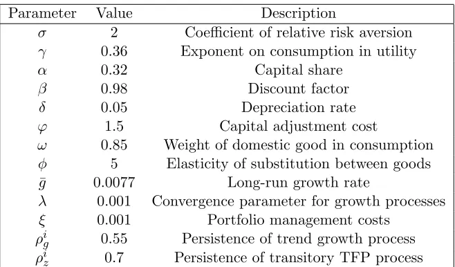
countries minus the U.S.8 The calibration is quarterly. Table 2 presents the calibrated parameter
values. The parameters σ (coefficient of relative risk aversion), γ (weight on consumption versus
leisure in the utility function),α (capital share), β (discount factor), and δ (depreciation rate) are
the same as in Aguiar and Gopinath (2007) and are standard in the literature. We set ϕ(capital
adjustment cost) to 1.5, roughly halfway between the estimates in Aguiar and Gopinath (2007) for
8
Parameter Value Description
σ 2 Coefficient of relative risk aversion γ 0.36 Exponent on consumption in utility
α 0.32 Capital share
β 0.98 Discount factor
δ 0.05 Depreciation rate ϕ 1.5 Capital adjustment cost
ω 0.85 Weight of domestic good in consumption φ 5 Elasticity of substitution between goods ¯
g 0.0077 Long-run growth rate
λ 0.001 Convergence parameter for growth processes ξ 0.001 Portfolio management costs
ρi
g 0.55 Persistence of trend growth process
ρi
[image:13.612.142.471.81.274.2]z 0.7 Persistence of transitory TFP process
Table 2: Baseline calibration. Values forρi
g and ρiz are for specifications in which these parameters
are not estimated.
Canada and Mexico, and also close to the estimate in the working paper version of Nguyen (2011).9
Since we have a two-good model, we also have two parameters governing households’ preferences
over home and foreign goods. Following Coeurdacier et al. (2010), we setω(the weight on domestic
goods in the consumption basket) to 0.85, corresponding to a steady-state import share of 15%.
We set φ(the elasticity of substitution between goods) to 5, as in Coeurdacier (2009).10 We set ¯g
(steady-state growth rate) to 0.0077, which is the average quarterly growth rate of U.S. real GDP
over our sample period (1960.2–2009.4). We set the convergence parametersλandξ to 0.001, which
are standard in the literature (see, e.g., Nguyen (2011) and Guerrieri et al. (2005)).
When not estimated, we setρi
g (persistence of the trend growth process) to 0.55 andρiz
(persis-tence of the transitory component of TFP) to 0.7 for both the U.S. and the G6. These estimates are
from Nguyen (2011), based on U.S. data from 1960–2000. In some specifications, we also estimate
ρi
g and ρiz ourselves for the U.S. and the G6.
9
The working paper version of Nguyen (2011) was calibrated to quarterly data, as is our model. The published version was calibrated to annual data and reported a somewhat smaller estimate forϕ.
10
3.2 Impulse responses
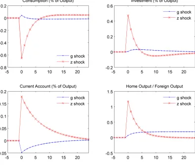
We consider a positive, 1% transitory shock and a positive, 0.1% trend shock to productivity in
the home country. Figure 2 shows the impulse responses for several key endogenous variables. In
response to a positive transitory shock, home country consumption falls on impact (as a share
of output). Agents understand that the shock is temporary: absent future shocks, output will
revert back to trend. In the language of the permanent income hypothesis, current income exceeds
permanent income. Optimal consumption smoothing requires that home households save a larger
share of their income, causing the consumption share to fall. In contrast, after a positive trend
shock, the consumption share rises. In this case, the shock is expected to have apermanent effect
on the level of output; moreover, the growth process has some persistence, so output will continue
to grow above trend for some time. Optimal consumption smoothing now dictates that home
households save a smaller share of their income and consume a higher share today. Investment
increases on impact in response to both shocks, though the response is more persistent – and much
less sharp on impact – with the trend shock.
In response to a positive trend shock, the higher consumption and investment shares together
push home’s current account into deficit. In this case, the home country needs to invest more in its
capital stock to take advantage of permanently higher productivity; but at the same time, home
households are less willing to save, since they expect future income to be higher than current income.
The solution, of course, is to borrow the difference from foreigners, who finance the home country’s
new investment. In contrast, a positive transitory shock pushes consumption and investment in
opposite directions. The home country still increases investment on impact, but home households
are also willing to save more. In our baseline calibration, the consumption share falls by more than
the investment share increases, creating a current account surplus.11
Note that home’s output grows more quickly than foreign output in response to both shocks. It
follows that the current account is countercyclical in response to a trend shock and procyclical in
response to a transitory shock in the baseline calibration. GMM estimation will attribute much of
the volatility of U.S. output to trend rather than transitory productivity shocks, as we demonstrate
11
in the next section.
4
Quantitative Results
We identify the parameters governing the trend and transitory shock processes using GMM
esti-mation.12 We present results based on quarterly data from 1960.2–2009.4.13
We estimate the model using data on U.S. and G6 macro variables. Data on U.S. output,
consumption, investment, and the current account is from the BEA. G6 data is from the OECD
database. Appendix D contains details on the data.
We estimate several specifications of the model with trend and transitory shocks. For
compar-ison, we also estimate the model with transitory shocks only and with trend shocks only.
4.1 Trend and transitory shocks
In the spirit of Aguiar and Gopinath (2007), we estimate several different specifications – starting
with a parsimonious set of moment conditions and building up to a richer specification. In the
first specification, we fix the persistence parameters at their calibrated values (ρH
g = ρFg = 0.55
and ρH
z = ρFz = 0.7) and estimate only the volatilities of the shocks: σgH, σzH, σgF, and σzF. The
target moments are the volatilities of Hodrick-Prescott filtered output and consumption in both
regions: σ(yus),σ(cus),σ(yg6), andσ(cg6).14 At each iteration of the GMM procedure, we run 200
simulations of 500 periods each and compute the average and standard deviation of the resulting
moments.
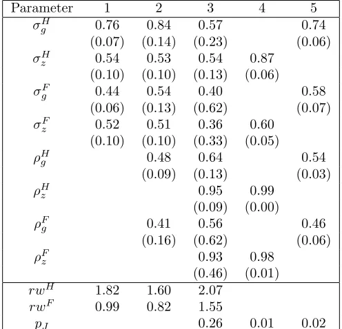
Table 3, Column 1 presents the estimates from this specification. The estimation assigns a
significant volatility to trend shocks in both regions. However, a complete comparison must also
take account of the persistence parameters and the labor-augmenting nature of the growth process.
Following Aguiar and Gopinath (2007), we compute a measure of the random walk component of
the (log) Solow residual:
12
See Burnside (1999) for a detailed description of the GMM technique with applications to macro models.
13
Results are qualitatively similar if the model is estimated over 1980.1-2009.4. Appendix C presents these results.
14
Output and consumption are nonstationary in the model, hence the need for some kind of detrending or filtering. The model solution produces decision rules for detrended output and consumption, ˆyH
t and ˆcHt . We use these decision rules to simulate a time path for detrended output and consumption, then use the realizations of the (cumulative) growth shocks to recover the levelsyH
Parameter 1 2 3 4 5 σH
g 0.76 0.84 0.57 0.74
(0.07) (0.14) (0.23) (0.06) σH
z 0.54 0.53 0.54 0.87 (0.10) (0.10) (0.13) (0.06) σF
g 0.44 0.54 0.40 0.58
(0.06) (0.13) (0.62) (0.07) σF
z 0.52 0.51 0.36 0.60 (0.10) (0.10) (0.33) (0.05) ρH
g 0.48 0.64 0.54
(0.09) (0.13) (0.03) ρH
z 0.95 0.99
(0.09) (0.00) ρF
g 0.41 0.56 0.46
(0.16) (0.62) (0.06) ρF
z 0.93 0.98
(0.46) (0.01) rwH 1.82 1.60 2.07
rwF 0.99 0.82 1.55
[image:17.612.182.430.168.407.2]pJ 0.26 0.01 0.02
Table 3: Estimated parameter values using GMM estimation (1960.2–2009.4). Estimated values for standard deviations are expressed in percentage terms. Standard errors are in parentheses. rwi
is the variance of the random walk component of the (log) Solow residual divided by the variance of the (log) Solow residual. For overidentified models, pJ is the p-value of the J statistic for the
overidentification test. A value less than 0.05 indicates that we can reject the model at the 5% level. The target moments for Specification 1 are the volatilities of HP-filtered output and consumption in each region{σ(yus),σ(cus),σ(yg6),σ(cg6)}. The target moments for Specification 2 include all the
target moments of Specification 1, plus the correlation of HP-filtered consumption with output in each region{ρ(yus, cus), ρ(yg6, cg6)}. The target moments for Specifications 3, 4, and 5 include all
the target moments from Specification 2, plus the volatilities of first-differenced (unfiltered) output in each region, {σ(∆yus), σ(∆yg6)}; the correlation of HP-filtered current-account-to-GDP with
output,{ρ(yus, caus)}; the first-order autocorrelation of HP-filtered output in each region,{ρ(yus),
ρ(yg6)}; and the first-order autocorrelation of first-differenced (unfiltered) output in each region,
{ρ(∆yus), ρ(∆yg6)}. Specification 4 sets σgH =σFg = 0. Specification 5 sets σHz =σzF = 0. When
not estimated, we set ρH
Moment Data 1 2 3 4 5 σ(yus) 1.53 1.53 1.53 1.42 1.29 1.22
(0.11) (0.11) (0.11) (0.09) (0.11) σ(cus)/σ(yus) 0.81 0.81 0.81 0.82 0.78 0.95
(0.02) (0.02) (0.03) (0.01) (0.02) σ(ius)/σ(yus) 4.63 2.24 2.23 2.21 2.24 2.12
(0.05) (0.05) (0.05) (0.03) (0.06) σ(yg6) 1.12 1.12 1.12 0.94 0.93 0.89
(0.07) (0.07) (0.07) (0.07) (0.07) σ(cg6)/σ(yg6) 0.71 0.71 0.71 0.80 0.70 0.95
(0.03) (0.03) (0.04) (0.01) (0.03) σ(ig6)/σ(yg6) 2.41 2.46 2.44 2.41 2.32 2.31
(0.10) (0.09) (0.12) (0.05) (0.11) σ(caus) 0.12 0.54 0.49 0.51 0.19 0.50
(0.03) (0.03) (0.03) (0.01) (0.03) ρ(yus, cus) 0.87 0.84 0.87 0.84 1.00 0.89
(0.02) (0.02) (0.02) (0.00) (0.01) ρ(yus, ius) 0.91 0.94 0.95 0.94 0.96 0.93
(0.01) (0.01) (0.01) (0.00) (0.01) ρ(yus, caus) -0.43 -0.12 -0.18 -0.11 -0.65 -0.30
(0.06) (0.06) (0.06) (0.04) (0.04) ρ(yg6, cg6) 0.82 0.77 0.82 0.80 0.99 0.87
(0.03) (0.03) (0.03) (0.00) (0.02) ρ(yg6, ig6) 0.91 0.86 0.87 0.81 0.93 0.79
(0.02) (0.01) (0.03) (0.01) (0.03) σ(∆yus) 0.87 0.97 1.00 0.84 0.99 0.63
(0.04) (0.04) (0.03) (0.03) (0.03) σ(∆yg6) 0.76 0.80 0.82 0.57 0.69 0.48
(0.03) (0.03) (0.02) (0.02) (0.02) ρ(yus) 0.86 0.81 0.80 0.85 0.74 0.92
(0.02) (0.02) (0.02) (0.03) (0.01) ρ(yg6) 0.85 0.73 0.72 0.83 0.74 0.91
(0.03) (0.03) (0.02) (0.03) (0.01) ρ(∆yus) 0.34 0.22 0.21 0.30 0.02 0.67
(0.04) (0.04) (0.04) (0.05) (0.03) ρ(∆yg6) 0.46 0.04 0.04 0.24 0.01 0.57
[image:18.612.160.452.152.595.2](0.05) (0.05) (0.05) (0.05) (0.03)
rw= (1−α)
2σ2
g/(1−ρg)2
[2/(1 +ρz)]σz2+ [(1−α)2σg2/(1−ρ2g)]
(14)
Equation (14) is based on a Beveridge-Nelson decomposition of the Solow residual (Beveridge
and Nelson, 1981).15 The resulting value for the U.S. is 1.82. This is significantly higher than the
random walk components of both Canada (0.37) and Mexico (0.96), as estimated by Aguiar and
Gopinath (2007). rw is also considerably higher for the U.S. than for the G6 (0.99), according to
our estimation. We find it striking that so much of the variation in U.S. TFP can be attributed to
trend shocks, which are commonly thought of as an emerging-market phenomenon.
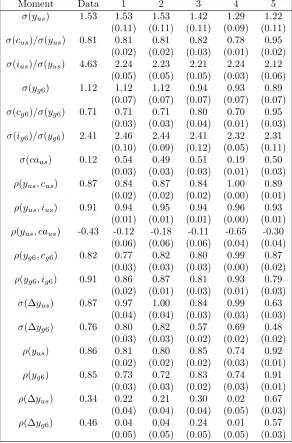
Table 4 compares business cycle moments across model and data. Specification 1 matches the
four target moments exactly. It also predicts a countercyclical current account balance, although
the magnitude of the correlation is smaller in the model (-0.12) than in the data (-0.43). Note that
consumption is less volatile than output in the U.S. (σ(cus)/σ(yus) = 0.81). In this sense, the U.S.
differs from emerging economies, which tend to have relatively volatile consumption. Our results
show that strong trend shocks can be consistent with both a countercyclical current account and
low consumption volatility. The model somewhat underestimates the volatility of investment in the
U.S. and overestimates the volatility of the current account balance.
In Specification 2, we expand the set of target moments to also include the correlation of
HP-filtered consumption with output in both regions, {ρ(yus, cus), ρ(yg6, cg6)}, and we estimate two
more parameters: ρH
g and ρFg. The main quantitative results are unchanged. In particular, the
estimation still predicts a high rw for the U.S. (1.60) and a moderately countercylical current
account balance (-0.18).
Specification 3 is the richest specification we consider, and our preferred one. We now estimate
all the parameters governing the trend and transitory shock processes: σH
g , σHz ,σFg,σFz, ρHg , ρHz ,
ρF
g, andρFz. We use 13 target moments: the volatilities of HP-filtered output and consumption in
each region, {σ(yus), σ(cus), σ(yg6), σ(cg6)}; the volatilities of first-differenced (unfiltered) output
in each region, {σ(∆yus), σ(∆yg6)}; the correlation of HP-filtered consumption with output in
15
each region, {ρ(yus, cus), ρ(yg6, cg6)}; the correlation of HP-filtered current-account-to-GDP with
output,{ρ(yus, caus)}; the first-order autocorrelation of HP-filtered output in each region,{ρ(yus),
ρ(yg6)}; and the first-order autocorrelation of first-differenced (unfiltered) output in each region,
{ρ(∆yus), ρ(∆yg6)}. The estimation continues to assign a significant volatility to trend shocks
in both regions, and the rw statistic for the U.S. is quite high (2.07). With 13 target moments
and 8 parameters to estimate, the model is now overidentified, so we can test the overidentifying
restrictions. The p-value of the J statistic is 0.26, so we cannot reject the model at any of the
standard confidence levels. Although some of the parameters for the G6 are not very precisely
estimated, all of the estimates for the U.S. are reasonably precise.
The model moments match the data reasonably well (Table 4, Column 3). The model continues
to predict a moderately countercyclical current account balance (-0.11). Most of the other moments
are a good match. The main exceptions are the volatility of investment in the U.S. (underestimated)
and the volatility of the current account (overestimated). This specification offers a closer match
to the autocorrelations of first-differenced output than the previous two specifications did.
4.2 Transitory shocks only
Next, we ask what happens when we turn the trend shocks off. In Specification 4, we fix σH g =
σF
g = 0 and estimate σzH, σzF, ρHz , and ρFz. The target moments are the same as in Specification
3. Interestingly, the estimation now assigns a very high value to ρH
z (0.99), the persistence of
the transitory TFP process.16 Roughly speaking, the model now “wants” the transitory shock to
be permanent. Even more interesting, the model now predicts a strongly countercyclical current
account (-0.62). This appears to go against the intuition from impulse response functions in Section
3, where we argued that the current account tends to increase after a positive transitory shock.
However, when the transitory TFP process is extremely persistent, this result is overturned, and
a positive transitory shock can lead to a decline in the current account. Effectively, the transitory
shock behaves more like a permanent shock whenρH
z is very high.17
16
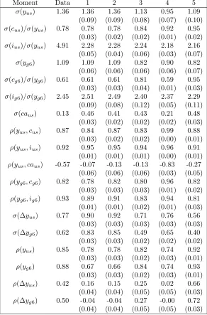
When estimated over 1980.1–2009.4, this result is even more dramatic: the estimation pinsρHz arbitrarily close to 1, the upper bound of the valid range of values for this parameter. Appendix C contains estimation results over 1980.1–2009.4.
17
This result turns out to be highly sensitive to the exact value of ρz. We also estimated a specification of the model where we fixed ρH
Overall, Specification 4 (transitory shocks only) does not fit the data as well as Specification 3
(trend and transitory shocks). In particular, Specification 4 predicts a nearly lockstep correlation
between HP-filtered consumption and output in both regions. The model also underestimates
the autocorrelation of HP-filtered output and the autocorrelation of first-differenced (unfiltered)
output. The p-value of theJ statistic is 0.01, indicating that we can reject the model at the 5%
level.
4.3 Trend shocks only
Specification 5 shuts off the transitory shocks. We now fix σH
z = σFz = 0 and estimate σgH, σgF,
ρH
g , andρFg. The target moments are the same as in Specifications 3 and 4. Specification 5 again
predicts a countercyclical current account (-0.30). However, relative to Specification 3 (trend and
transitory shocks), it underestimates the volatility of output and overestimates the volatility of
consumption in each region. Specification 5 also underestimates the volatility of first-differenced
output and overestimates the autocorrelation of first-differenced output. The p-value of the J
statistic is 0.02, again suggesting that we can reject the model at the 5% level.
5
Conclusion
Previous research has identified trend growth shocks to productivity as a possible driver of
counter-cyclical external balances in emerging market countries. We argue that trend shocks can also help
explain the countercyclical U.S. current account. Our approach has been to estimate a structural
open economy macro model with trend and transitory productivity shocks. The specification that
best matches the data assigns a large role to trend shocks. When estimated with transitory shocks
alone, the model can produce a countercyclical current account only if the transitory TFP process
is extremely persistent. While the simple RBC model considered here matches the data reasonably
well, it does tend to underestimate the volatility of investment and overestimate the volatility of the
current account. We speculate that adding financial frictions and shocks affecting firms’ borrowing
ability could improve the fit of the model, as suggested by Garcia-Cicco et al. (2010) and others.
Appendix
A
First-order conditions
The first-order conditions of the representative firm in countryiare:
wit= (1−α)y
i t
li t
(15)
1 +ϕ
ki t+1
ki t
−eg¯
=
Et
"
mit+1,t
pi t+1 pi t ( αy i t+1 ki t+1
+ 1−δ+ϕ 2 ki t+2 ki t+1 2
− eg¯2
!)#
(16)
The first-order conditions of the representative household in countryiare:
ci,t−i ci,it =
1−ω ω
pi t
p−i t φ (17) ci t γ = pi
twti
pi,ct
1−li t
1−γ
(18)
ui c,t
pi,ct
1 +ξb
i t+1
ΓH t
=Et
"
β u
i c,t+1
pi,ct+1
!
rt
#
(19)
where uic,t≡ h
ciγt (1−li t)1−γ
i1−σ
ci t
B
Detrending and Equilibrium
To solve the model using locally accurate solution techniques, it is necessary to express it in
de-trended form. For any (trending) variable xt, letxbt ≡xt/ΓHt−1 be its detrended counterpart. The
following variables have a stochastic trend and need to be detrended: yi
t,kti,dit,wti,bit,cit, and c i,j t .
The remaining variables are already stationary. In what follows, it is useful to define the following
ht≡
ΓH t
ΓH t−1
=egHt πλ
t
The production functions can then be written as follows:
b
yH t =ez
H t bkHα
t lHt ht
1−α
(20)
b
ytF =eztFbkF α
t
lFt egFt π1−λ
t
1−α
(21)
The law of motion for capital can be written:
b
kit+1ht=xbti+ (1−δ)bkit−
ϕ 2
b
ki t+1ht
b
ki t
−eg¯
!2
b
kit (22)
The household budget constraint can be written:
pitwbitlti+dbit+rt−1bbit=p i,c
t bcit+bbit+1ht+
ξ 2
bbit+12ht (23)
The intertemporal first-order condition for the representative household can be written:
ui
b
c,t
pi,ct
1 +ξbbi t+1
=Et
"
β u
i
b
c,t+1
pi,ct+1
!
hγ(1t −σ)−1rt
#
(24)
where uibc,t≡ h
b
ciγt (1−li t)1−γ
i1−σ
b
ci t
1 +ϕ bk
i t+1ht
b
ki t
−e¯g
!
=
Et
mit+1,t
pi t+1 pi t α b yi t+1 b ki t+1
+ 1−δ+ϕ 2
bkt+2i ht+1
b
ki t+1
!2
− e¯g2
(25)
The stochastic discount factor can be written:
mit+1,t=β u
i b c,t+1 ui b c,t !
pi,ct pi,ct+1
!
hγ(1t −σ)−1 (26)
The market-clearing conditions (11) and (12), the expression for the consumption basket (5),
the expression for shareholder proceeds (3), the expression for the current account (13), and the
remaining first-order conditions can be written in detrended form simply by replacing each trending
variablext with its detrended counterpart,xbt.
An equilibrium is a sequence of prices {pi
t,wbit, rit}, capital stocks {bkti}, labor {lti}, output{byit},
consumption {bci,jt }, and bond holdings {bbi
t} such that (i) goods and asset markets clear, and (ii)
households and firms in both countries behave optimally, taking prices as given.
C
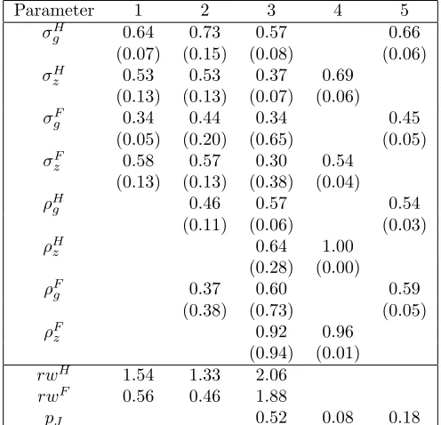
Estimation results over 1980.1–2009.4
Tables 5 and 6, below, present results from estimating the model over the time period 1980.1–
2009.4. The baseline calibration is the same as in Table 2, except that ¯g is set to 0.0067 to match
the quarterly growth rate of U.S. output over this time period.
D
Data
This appendix describes the data used in our estimation exercises. Data is quarterly, from 1960.2–
2009.4. We take output, consumption, and investment from the BEA for the U.S., and from the
OECD “StatExtracts” database for the G6. We also get the U.S. current account balance from the
Parameter 1 2 3 4 5 σH
g 0.64 0.73 0.57 0.66
(0.07) (0.15) (0.08) (0.06) σH
z 0.53 0.53 0.37 0.69 (0.13) (0.13) (0.07) (0.06) σF
g 0.34 0.44 0.34 0.45
(0.05) (0.20) (0.65) (0.05) σF
z 0.58 0.57 0.30 0.54 (0.13) (0.13) (0.38) (0.04) ρH
g 0.46 0.57 0.54
(0.11) (0.06) (0.03) ρH
z 0.64 1.00
(0.28) (0.00) ρF
g 0.37 0.60 0.59
(0.38) (0.73) (0.05) ρF
z 0.92 0.96
(0.94) (0.01) rwH 1.54 1.33 2.06
rwF 0.56 0.46 1.88
[image:25.612.182.430.168.407.2]pJ 0.52 0.08 0.18
Table 5: Estimated parameter values using GMM estimation (1980.1–2009.4). Estimated values for standard deviations are expressed in percentage terms. Standard errors are in parentheses. rwi
is the variance of the random walk component of the (log) Solow residual divided by the variance of the (log) Solow residual. For overidentified models, pJ is the p-value of the J statistic for the
overidentification test. A value less than 0.05 indicates that we can reject the model at the 5% level. The target moments for Specification 1 are the volatilities of HP-filtered output and consumption in each region{σ(yus),σ(cus),σ(yg6),σ(cg6)}. The target moments for Specification 2 include all the
target moments of Specification 1, plus the correlation of HP-filtered consumption with output in each region{ρ(yus, cus), ρ(yg6, cg6)}. The target moments for Specifications 3, 4, and 5 include all
the target moments from Specification 2, plus the volatilities of first-differenced (unfiltered) output in each region, {σ(∆yus), σ(∆yg6)}; the correlation of HP-filtered current-account-to-GDP with
output,{ρ(yus, caus)}; the first-order autocorrelation of HP-filtered output in each region,{ρ(yus),
ρ(yg6)}; and the first-order autocorrelation of first-differenced (unfiltered) output in each region,
{ρ(∆yus), ρ(∆yg6)}. Specification 4 sets σgH =σFg = 0. Specification 5 sets σHz =σzF = 0. When
not estimated, we set ρH
Moment Data 1 2 3 4 5 σ(yus) 1.36 1.36 1.36 1.13 0.95 1.09
(0.09) (0.09) (0.08) (0.07) (0.10) σ(cus)/σ(yus) 0.78 0.78 0.78 0.84 0.92 0.95
(0.03) (0.02) (0.02) (0.01) (0.02) σ(ius)/σ(yus) 4.91 2.28 2.28 2.24 2.18 2.16
(0.05) (0.04) (0.06) (0.03) (0.07) σ(yg6) 1.09 1.09 1.09 0.82 0.90 0.82
(0.06) (0.06) (0.06) (0.06) (0.07) σ(cg6)/σ(yg6) 0.61 0.61 0.61 0.81 0.59 0.95
(0.03) (0.03) (0.04) (0.01) (0.03) σ(ig6)/σ(yg6) 2.45 2.51 2.49 2.40 2.37 2.29
(0.09) (0.08) (0.12) (0.05) (0.11) σ(caus) 0.13 0.46 0.41 0.43 0.21 0.48
(0.03) (0.02) (0.02) (0.02) (0.03) ρ(yus, cus) 0.87 0.84 0.87 0.83 0.99 0.88
(0.03) (0.02) (0.02) (0.00) (0.01) ρ(yus, ius) 0.92 0.95 0.95 0.94 0.96 0.91
(0.01) (0.01) (0.01) (0.00) (0.01) ρ(yus, caus) -0.57 -0.07 -0.13 -0.13 -0.83 -0.27
(0.06) (0.06) (0.06) (0.03) (0.05) ρ(yg6, cg6) 0.82 0.78 0.82 0.80 0.96 0.82
(0.03) (0.03) (0.03) (0.01) (0.02) ρ(yg6, ig6) 0.93 0.89 0.91 0.83 0.94 0.81
(0.01) (0.01) (0.02) (0.01) (0.03) σ(∆yus) 0.77 0.90 0.92 0.71 0.76 0.56
(0.03) (0.03) (0.03) (0.03) (0.03) σ(∆yg6) 0.62 0.83 0.85 0.49 0.65 0.40
(0.03) (0.03) (0.02) (0.02) (0.02) ρ(yus) 0.85 0.78 0.78 0.82 0.74 0.92
(0.03) (0.03) (0.02) (0.03) (0.01) ρ(yg6) 0.88 0.67 0.66 0.84 0.74 0.93
(0.03) (0.03) (0.02) (0.03) (0.01) ρ(∆yus) 0.42 0.16 0.15 0.25 0.02 0.66
(0.04) (0.04) (0.05) (0.05) (0.03) ρ(∆yg6) 0.50 -0.04 -0.04 0.27 -0.00 0.72
[image:26.612.160.452.152.595.2](0.04) (0.04) (0.05) (0.05) (0.03)
measure ‘CPCARSA’). Following Aguiar and Gopinath (2007), we HP-filter log real output, log real
consumption, and log real investment in both countries, as well as the ratio of the U.S. (nominal)
References
Aguiar, Mark and Gita Gopinath, “Emerging Market Business Cycles: The Cycle is the Trend,” Journal of Political Economy, 2007,115 (1), 69–102.
Angelopoulos, Konstantinos, George Economides, and Vangelis Vassilatos, “Do Institu-tions Matter for Economic FluctuaInstitu-tions? Weak Property Rights in a Business Cycle Model for Mexico,”Review of Economic Dynamics, 2011, 14(3), 511–531.
Backus, David, Patrick Kehoe, and Finn Kydland, “International Real Business Cycles,”
Journal of Political Economy, 1992, 100(4), 745–75.
Baxter, Marianne and Mario Crucini, “Business Cycles and the Asset Structure of Foreign Trade,” International Economic Review, 1995, 36(4), 821–854.
Beveridge, Stephen and Charles Nelson, “A New Approach to Decomposition of Economic Time Series into Permanent and Transitory Components with Particular Attention to Measure-ment of the ‘Business Cycle’,” Journal of Monetary Economics, 1981, 7(2), 151–74.
Blundell, Richard and Ian Preston, “Consumption Inequality And Income Uncertainty,”The Quarterly Journal of Economics, 1998,113 (2), 603–640.
Boz, Emine, Christian Daude, and Ceyhun Bora Durdu, “Emerging Market Business Cycles: Learning About the Trend,” Journal of Monetary Economics, 2011, Forthcoming.
Burnside, Craig, “Real Business Cycle Models: Linear Approximation and GMM Estimation,” 1999. Unpublished Manuscript, The World Bank Group.
Campbell, John and Angus Deaton, “Why Is Consumption So Smooth?,”Review of Economic Studies, 1989, 56(3), 357–73.
Chen, Kaiji, Ayse Imrohoroglu, and Selahattin Imrohoroglu, “A Quantitative Assessment of the Decline in the U.S. Current Account,” Journal of Monetary Economics, 2009, 56 (8), 1135–1147.
Christiano, Lawrence and Martin Eichenbaum, “Unit Roots in Real GNP: Do We Know, and Do We Care?,” Carnegie Rochester Conference Series on Public Policy, 1990, 32, 7–61.
Cochrane, John, “How Big is the Random Walk in GNP?,” Journal of Political Economy, 1988,
96 (5), 893–920.
Coeurdacier, Nicolas, “Do Trade Costs in Goods Markets Lead to Home Bias in Equities?,”
Journal of International Economics, 2009,77, 86–100.
, Robert Kollman, and Philippe Martin, “International Portfolios, Capital Accumulation and Foreign Asset Dynamics,”Journal of International Economics, 2010,80, 100–112.
Corsetti, Giancarlo and Panagiotis Konstantinou, “What Drives U.S. Foreign Borrowing? Evidence on the External Adjustment to Transitory and Permanent Shocks,”American Economic Review, 2011, Forthcoming.
Garcia-Cicco, Javier, Roberto Pancrazi, and Martin Uribe, “Real Business Cycles in Emerging Countries?,” American Economic Review, 2010,100 (5), 2510–31.
Gourinchas, Pierre-Olivier and H´el`ene Rey, “International Financial Adjustment,” Journal of Political Economy, 2007, 115.
Guerrieri, Luca, Dale Henderson, and Jinill Kim, “Investment-specific and Multifactor Pro-ductivity in Multi-Sector Open Economies: Data and Analysis,” International Finance Discussion Paper 828, Board of Governors of the Federal Reserve System 2005.
Heathcote, Jonathan and Fabrizio Perri, “Financial Autarky and International Business Cy-cles,” Journal of Monetary Economics, 2002, 49, 601–627.
Hoffmann, Mathias, Michael Krause, and Thomas Laubach, “Long-run Growth Expecta-tions and ‘Global Imbalances’,” Discussion Paper 01/2011, Deutsche Bundesbank 2011.
Lane, Philip and Gian Maria Milesi-Ferretti, “A Global Perspective on External Positions,” in Richard Clarida, ed.,G7 Current Account Imbalances: Sustainability and Adjustment, Chicago University Press, 2005.
and , “The External Wealth of Nations Mark II: Revised and Extended Estimates of Foreign Assets and Liabilities, 1970–2004,” Journal of International Economics, 2007, 73, 223–250.
Lumsdaine, Robin and David Papell, “Multiple Trend Breaks and the Unit-Root Hypothesis,”
Review of Economic Statistics, 1997, 79(2), 212–218.
Nguyen, Ha, “Valuation Effects with Transitory and Trend Productivity Shocks,” Journal of International Economics, 2011, Forthcoming.
Obstfeld, Maurice and Kenneth Rogoff, “The Unsustainable U.S. Current Account Position Revisited,” in Richard Clarida, ed., G7 Current Account Imbalances: Sustainability and Adjust-ment, Chicago University Press, 2005.
Ozbilgin, Husyein Murat, “Financial Market Participation and the Developing Country Busi-ness Cycle,” Journal of Development Economics, 2010, 92(2), 125–137.